Drafting Fantasy Football Teams: A Comparison Greedy Algorithms

Posted on September 7, 2015

Fantasy football is an increasingly popular game for American football fans. Coaches compete within a league, typically of friends or coworkers. The standard roster of starters includes 1 QB, 2 RB, 2 WR, 1 TE, 1 D/ST (defense/special teams), 1 K, and 1 F (flex: can usually be a WR, RB, or TE). Teams also have bench players (backups for when starters are struggling or on a bye week).

If you aren’t familiar with how fantasy football works, read more here. Even if you aren’t a big football fan, this is worth learning for the exciting strategy behind playing. From here on out, I will assume you have a basic working knowledge of the game.

There are a lot of week to week strategies that coaches employ to pick up the best players off the waiver wire or win week to week, but for now we will just focus on the draft.

Simple Greedy Algorithm

The simplest way to draft is to just pick the best available player. We will call this a greedy algorithm. There is no negative connotation implied here; it just describes the algorithm design: pick the best player available based on projected points.

As it turns out, this strategy isn’t too bad; better than wonky strategies like picking only Jets and Chargers players or only from teams capable of flight (both are strategies I've drafted against). Success in a draft is obviously not guaranteed. After all, only one person can draft the best team. As many seasoned coaches suspect, the lucky coaches with early picks (1-3 overall) are more likely to draft teams with the highest projections.

If you are the poor guy sitting in the back with the last pick, it seems like there’s nothing you can do. Even if you know who your opponents are picking, there is not a clear and intuitive way to leverage that information if you stick to just picking the best available. If only there was a way to take advantage of the knowledge of who other players are picking…and that’s where the predictive greedy algorithm comes in.

Predictive Greedy Algorithm

Let’s think through a modification of the simple greedy algorithm by considering the following situation. Let’s say (hypothetically) that you have the QB and WR positions open. Also, Peyton Manning is the best player available and he is worth 500 points, the next best player available is Calvin Johnson, projected to get 475 points. The simple greedy algorithm would tell you to pick Peyton because he is worth more points. When the next round comes around, Calvin Johnson is no longer available at WR so you have to “settle” on 375 from Brandon Marshall.

But wait, there’s more! Let’s also say 3 spots behind Peyton (in QBs) is Philip Rivers, a less popular choice, but still projected to get 425 points. And better yet, you know how you’re opponents pick so you know there is a high chance he’ll be available next round. So you can let Peyton Manning go to another team and pick up Calvin Johnson even though he doesn’t have the highest points available, then get Phillip Rivers the next round(Peyton will surely be gone). Some simple math later, you drafted two players worth a combined 475+425=900 points (Johnson and Rivers) instead of 500+375=875 (Manning and Marshall), because you were able to predict what your opponents were going to do, and exploited it.

With that example in mind, let's formally define our new greedy algorithm. Each pick you will follow these steps:

Determine the best available player and simulate that you pick him
Determine the best available player at every other position
Simulate other coaches picking for a round until the pick comes back to you
Once again, determine the best available player at every position
Calculate the position with the highest decrease in points and pick that player

There are some obvious shortcomings to this highly trivialized situation, namely the lack of information. You will never know exactly who you’re opponents are going to pick, and risking big by drafting lower rated players earlier can be dangerous. However, in our academically predictable environment, this strategy proves to be quite fruitful.

Comparison

We are going to simulate 66 different drafts: 6-16 person leagues (by 2’s) with everyone picking with the simple greedy strategy except for one person, who will pick with the predictive greedy algorithm. The code is largely unexciting bookkeeping so I won’t walk through it, but you can find it on GitHub.

As expected, the predictive greedy algorithm is quite successful, particularly in larger drafts and for players in the middle of the draft order.

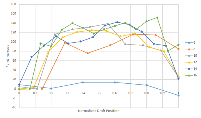
Point increase from using predictive greedy strategy compared to simple greedy strategy

Coaches who picked following this strategy picked the team with the highest projected points 89% of the time.

Other Considerations

This is obviously a drastic oversimplification of the drafting problem, namely because we know our opponents strategy. In reality, coaches’ picks are more sporadic. Some coaches employ strategies like picking 3 RBs in their first 3 rounds, others pick players heavily from their favorite teams.

Regardless of how your league tends to pick, a key to success is to get out front of these trends right before they happen (and not too early). We can see the importance of this in the chart below.

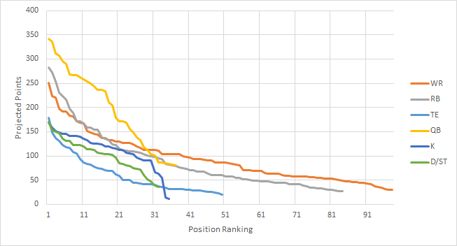
Projected points plotted against ranking (by position)

Each position has diminishing point value (the slope flattens out) as you go further out in the rankings, some faster than others. You want to pick anytime when the slope is steep, but on the front end (you don't want to pick after the major drop offs). But not all positions are picked at the same time, and this varies by league. In some leagues, quarterbacks go in the 1st round, in some not till the 5th - some leagues pick defenses in the 5th round and some pick defenses in the 8th round. If you know other coach's tendencies, you can get out in front of these major drop offs and take advantage of them.

This overlooks a few other important details - one of which is the bye week problem. Each player has a bye week some time from Week 4 to Week 11 in the 17 week season. Some coaches hedge against this by spreading out the bye weeks among their team – others try to get all the bye weeks at the same time so their team takes only one bad loss.

Another overlooked assumption comes from picking bench players. Consider a 6-team league. There are far more than six QBs that are fairly evenly matched and good enough to start on a fantasy team. Therefore in this simulation, a coach who waits until the last pick to draft the QB does not suffer too much in points lost. However, in reality, some coaches pick their backup QB quite early; some even draft a backup before they fill in all of their starting positions. This decision-making process is hard to predict in these simulations.

With all the assumptions that have gone into this analysis, it’s unlikely that a coach could replicate this success without a little bit of luck and lot of predictable behavior from their opponents. If you did have this information (looking at you ESPN), there is a lot of potential to take this in exciting new directions.

More Approximations for Trigonometric Functions with the Binomial Series

Posted on August 31, 2015

In this post, we will create a new set of approximations for sine and cosine that utilize the binomial series. Before you go any further, you may want to read this previous post where we walk through the binomial series and comparisons to the Maclaurin series.

Derivation

We are going to exploit Euler's formula with a twist. To refresh your memory, here's Euler's Formula. \begin{equation} \cos(\theta)+i\sin(\theta)=e^{i\theta} \end{equation} Now let's employ one of the older tricks in the book, adding and subtracting one from the same expression: \begin{equation} \cos(\theta)+i\sin(\theta)=\left[(e-1)+1\right]^{i\theta}. \end{equation} Now we have a binomial raised to a power. Once again, we will use known values and the binomial series to generate approximations for sine and cosine.

Fine Tuning For Approximation

In its current form this would almost be enough for decent approximations. However, closely tied to the accuracy of an approximation is the convergence rate of the series. To improve convergence, we want to make one of the terms small relative to the other term. Is there anything we can do here?

As a matter of fact, yes. We will employ a second manipulation - multiplying and dividing by the same number (inside and outside of the parentheses). Consider the updated equation \begin{equation} \cos(\theta)+i\sin(\theta)=a^i\cdot\left[\left(\displaystyle\frac{e}{a^{1/\theta}}-1\right)+1\right]^{i\theta}. \end{equation} If you need to, convince yourself that this is still valid. Now, to build a valid approximation, we need $\displaystyle\frac{e}{a^{1/\theta}}-1$ to be small for a range of values. In our previous post, we determined that you need a range of $\pi/4$ for sine and cosine, which could be extrapolated out to encompass all values.

Ideally we would just pick the range $[0,\pi/4]$, with which a value of $a=e^{\pi/8}$ would be a good place to center the approximation. However, If $\theta=0$, the expression \begin{equation} {(e^{\pi/8})^{1/0}}-1 \end{equation} is not defined (although the limit appears to exist).

On the other side of the range, at $\theta=\pi/4$, the expression becomes \begin{equation} \displaystyle\frac{e}{(e^{\pi/8})^{4/\pi}}-1=e^{1/2}-1\approx.64 \end{equation} which is enough for convergence, but maybe not optimal.

On the other hand, if we made the range $[2\pi,2\pi+\pi/4]$ with $a=2\pi+\pi/8$, then our bounding values are roughly $\approx\pm.06$ which will give us much better convergence. Due to the nature of this equation, rapidly increasing our range - for example, the range $[100\pi,100\pi+\pi/4]$ - has rapidly diminishing gains, and improved convergence will be offset by roundoff error elsewhere.

Implementing Approximations

An example of this code is (written for MATLAB) is

iterations=14;
start=2*pi;
range=pi/4;
increment=.001;

theta=start:increment:(start+range);

a=exp(start+range/2);
z=1i.*theta;
w=exp(1)./a.^(1./theta)-1;

approx=zeros(1,length(theta));

for i=iterations:-1:1
    approx=1+approx.*(w.*(z-i+1)/i);
end
         
approx=approx*a.^(1i);

You can plot the error with the following code

error=real(approx)-cos(theta);
figure; 
h=semilogy(theta,abs(error));
outfilename=sprintf('cos_error_%d_iter',iterations);
saveas(h, outfilename, 'png');

error=imag(approx)-sin(theta);
figure; 
h=semilogy(theta,abs(error));
outfilename=sprintf('sin_error_%d_iter',iterations);
saveas(h, outfilename, 'png');

Error Plots

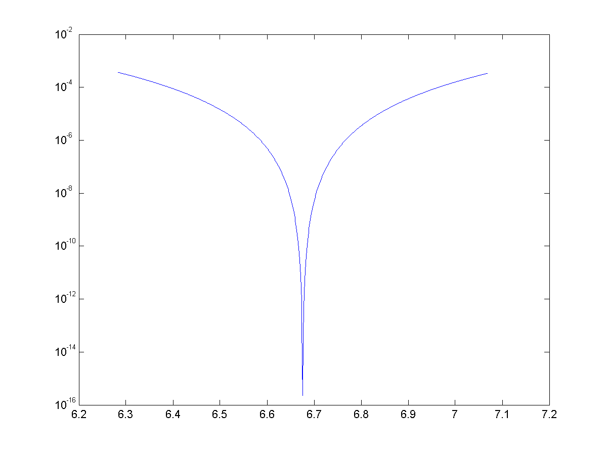
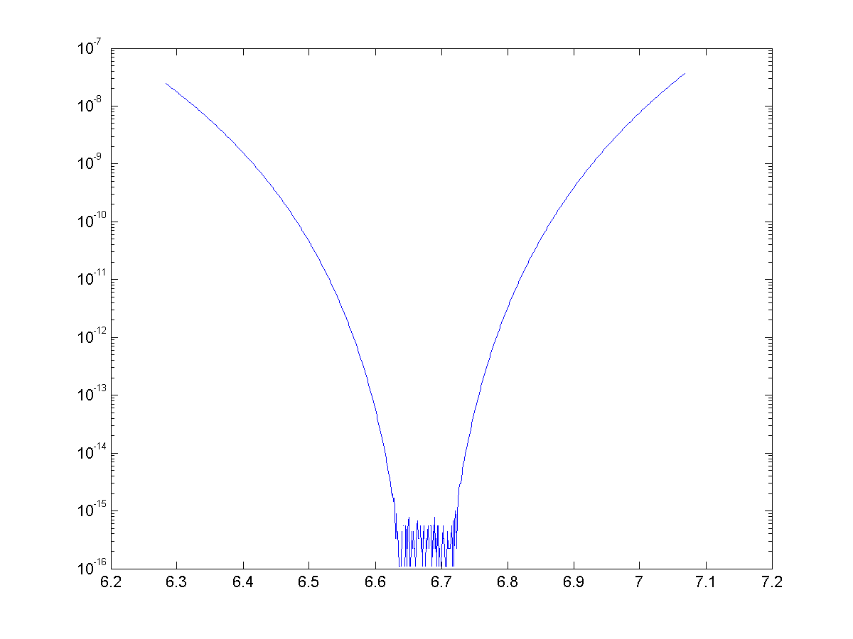
See below for the error for approximations for cosine with 4, 8, 12, and 14 terms. With 14 terms, we are more or less bounded by machine precision (~15 significant figures)

Error plot for $\cos(\theta)$ approximated with 4 terms on the range $\theta=[2\pi,2\pi+\pi/4]$

Error plot for $\cos(\theta)$ approximated with 8 terms on the range $\theta=[2\pi,2\pi+\pi/4]$

Error plot for $\cos(\theta)$ approximated with 12 terms on the range $\theta=[2\pi,2\pi+\pi/4]$

Error plot for $\cos(\theta)$ approximated with 14 terms on the range $\theta=[2\pi,2\pi+\pi/4]$

Error plot for $\sin(\theta)$ approximated with 14 terms on the range $\theta=[2\pi,2\pi+\pi/4]$

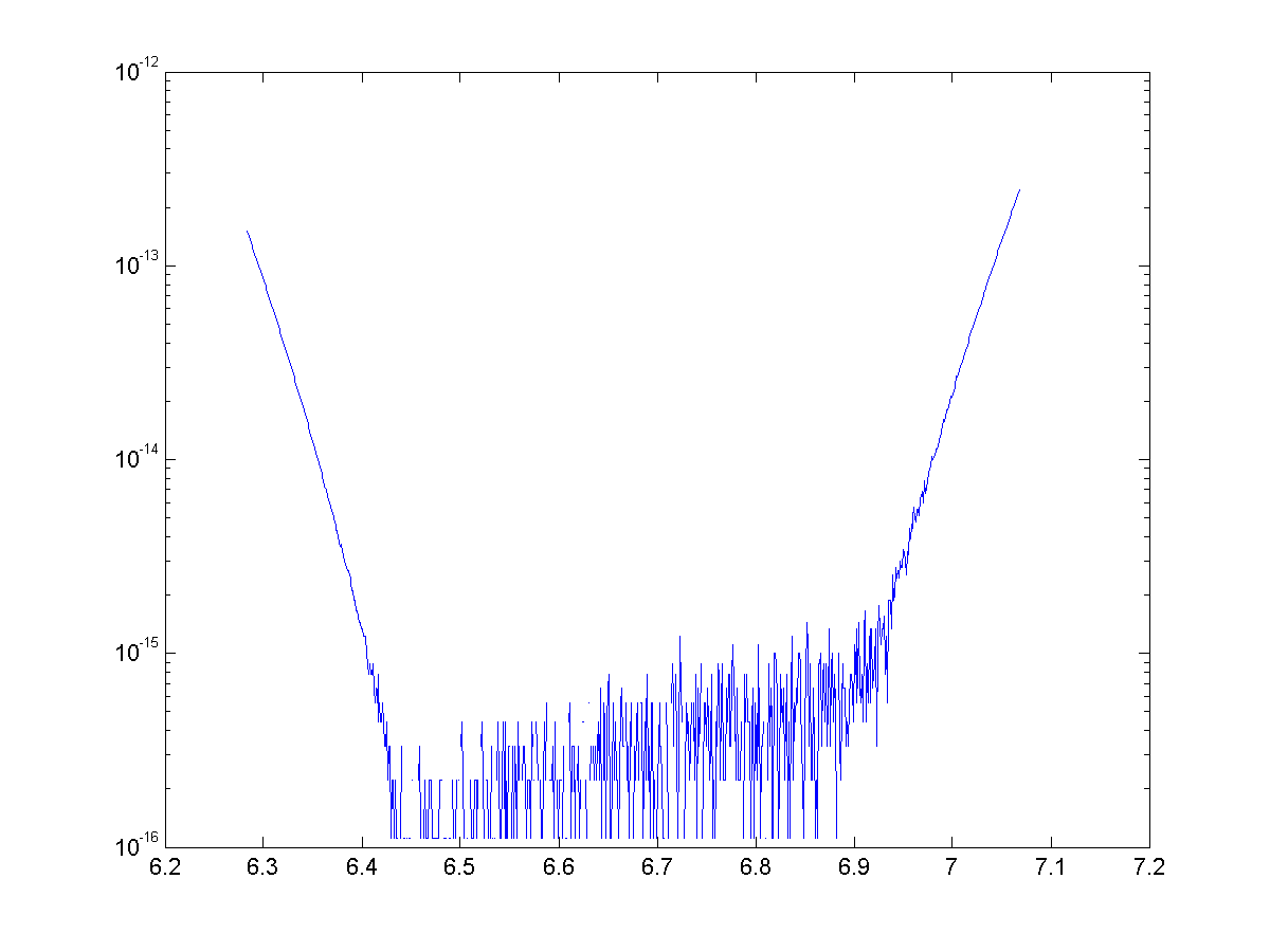
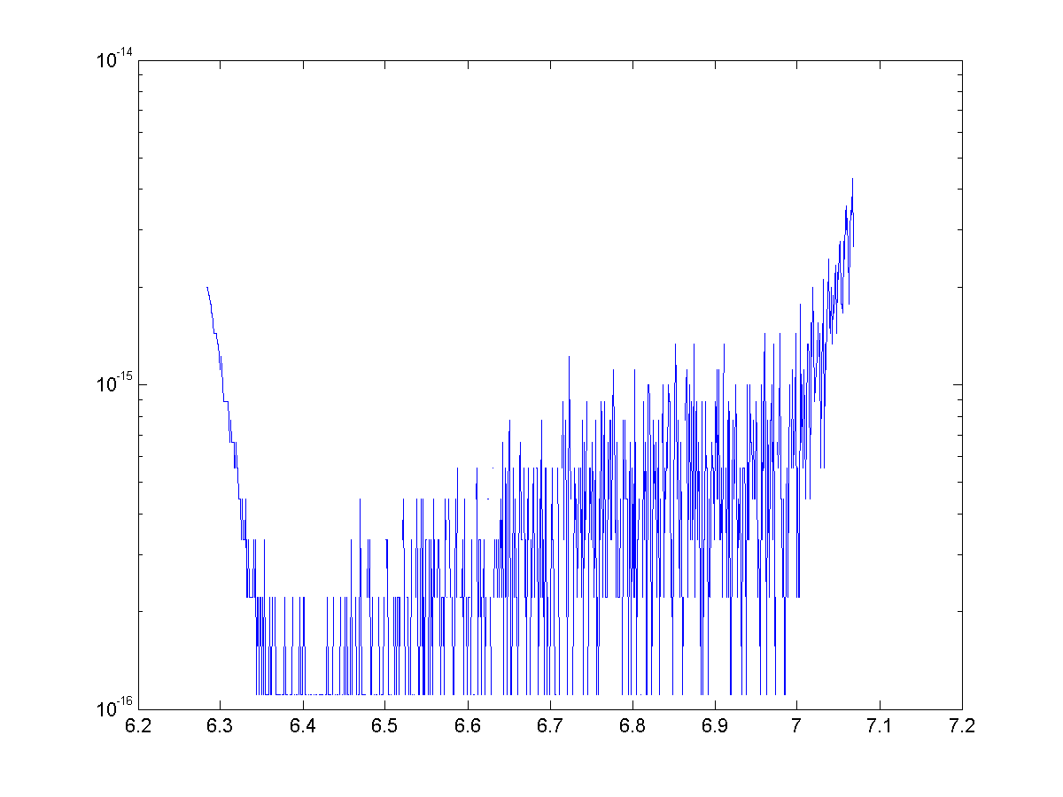
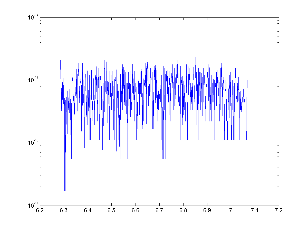
Once again we have generated some exciting looking, but nonetheless useless approximations. We were able to use binomial theorem and some trickery to generate approximations with great accuracy, but once again they are nowhere near as speedy to calculate as the Maclaurin series.

Contents

Categories

Archives