Newton’s Method for Polynomials
Posted on April 14, 2018
Newton’s Methods is a useful tool for finding the roots of real-valued, differentiable functions. A drawback of the method is its dependence on the initial guess. For example, all roots of a 10th degree polynomial could be found with 10 very good guess. However, 10 very bad guesses could all point to the same root.
In this post, we will present an iterative approach that will produce all roots. Formally
Newton's method can be used recursively, with inflection points as appropriate initial guesses, to produce all roots of a polynomial.
Motivation
While working through the Aero Toolbox app, I needed to solve a particular cubic equation (equation 150 from NACA Report 1135, if you're interested).
I needed to find all 3 roots. The cubic equation is well known, but long and tedious to code up. I had already been implementing Newton’s Method elsewhere in the app and wanted to use that. The challenge though, as is always the challenge with using Newton’s Method on functions with multiple roots is robustly finding all of them.
This particular cubic was guaranteed to have three distinct roots. The highest and lowest were easy; I was solving for the square of the sine of particular angles so $0$ and $1$ are good starting points. The middle root was not so easy. After some brainstorming, I took a stab at a possible guess: the inflection point. Low and behold, it (without fail) always converged the middle root.
Delving Further
So why did the inflection point always converge to the middle root? Let's explore!
We'll start with a simple example: a polynomial with unique, real roots. The root is either identical to the inflection point, to the left of it, or to the right of it.
Assume WLOG that the derivative is positive in this region. There will always be a root in between the inflection point and the local min/max to each side (This statement requires proof, which will of course be left to the reader ;) ). Let's examine all three cases.
Case 1: Inflection Point is a root
You are at a root, so Newton's Method is converged. Both the function $p$ and its derivative $p'$ are $0$, so as long as your implementation avoids division by zero or erratic behavior close to $\frac{0}{0}$, you're in the clear.
Case 2: Root to the left of the inflection point
The slope will flatten out to the left of the inflection point, therefore the tangent line will intersect the $x$-axis before $p$ does. That means Newton's Method will not overshoot the root. In subsequent guesses, this same pattern will hold.
Consider an example in the graph below, $p(x)=-\frac{x^3}{6}+x+0.85$, shown in blue. In the graph below, the tangent line is shown in purple. The intersection of the tangent line and the $x$-axis is the updated guess.
Source: Wolfram Alpha
Case 3: Root to the right of the inflection point
The logic is the same, but with signs reversed. The root is to the right of the inflection point. All guesses will move right monotonically without overshooting the root.
Consider an example in the graph below of a different polynomial, $p(x)=-\frac{x^3}{6}+x-0.85$, shown in blue. In the graph below, the tangent line is shown in purple. The intersection of the tangent line and the $x$-axis is the updated guess.
Source: Wolfram Alpha
Generalizing to Higher Order Polynomials
This method can be generalized to higher orders in a recursive fashion. For an $n$th order polynomial $p$ we can use the roots 2nd derivative $p’’$ (degree $n-2$) as starting guesses for the roots of $p$. To find the roots of $p’’$, you need the roots of $p’’’’$ and so on. Also, as part of the method, you need $p’$. Therefore, all derivatives of the polynomial are required.
Two functions are required. First, a simple implementation of Newton's method
def newton_method(f, df, g, deg):
    max_iterations = 100
    tol = 1e-14
    for i in xrange(max_iterations):
        fg = sum([g ** (deg - n) * f[n] for n in xrange(len(f))])
        dfg = float(sum([g ** (deg - n - 1) * df[n] for n in xrange(len(df))]))
        if abs(dfg) < 1e-200:
            break
        diff = fg / dfg
        g -= diff
        if abs(diff) < tol:
            break
    return g
The second part is iteration
def roots_newton(coeff_in):
    ndof = len(coeff_in)
    deg = ndof - 1
    coeffs = {}
    roots = [([0] * row) for row in xrange(ndof)]

    # Make coefficients for all derivatives
    coeffs[deg] = coeff_in
    for i in xrange(deg - 1, 0, -1):
        coeffs[i] = [0] * (i+1)
        for j in range(i+1):
            coeffs[i][j] = coeffs[i + 1][j] * (i - j + 1)

    # Loop through even derivatives
    for i2 in xrange(ndof % 2 + 1, ndof, 2):
        if i2 == 1:   # Base case for odd polynomials
            roots[i2][0] = -coeffs[1][1] / coeffs[1][0]
        elif i2 == 2: # Base case for even polynomials
            a, b, c = coeffs[2]
            disc = math.sqrt(b ** 2 - 4 * a * c)
            roots[2] = [(-b - disc) / (2 * a), (-b + disc) / (2 * a)]
        else:
            guesses = [-1000.] + roots[i2 - 2] + [1000.] #Initial guesses of +-1000
            f = coeffs[i2]
            df = coeffs[i2 - 1]
            for i, g in enumerate(guesses):
                roots[i2][i] = newton_method(f, df, g, i2)
    return roots[-1]
This method will also work for polynomials with repeated roots. However, there is no mechanism for finding complex roots.
Comparison to Built-in Methods
The code for running these comparisons is below.#repeated roots ps = [[1, 2, 1], [1, 4, 6, 4, 1], [1, 6, 15, 20, 15, 6, 1], [1, 8, 28, 56, 70, 56, 28, 8, 1], [1, 16, 120, 560, 1820, 4368, 8008, 11440, 12870, 11440, 8008, 4368, 1820, 560, 120, 16, 1], #unique roots from difference of squares [1, 0, -1], [1, 0, -5, 0, 4], [1, 0, -14, 0, 49, 0, -36], [1, 0, -30, 0, 273, 0, -820, 0, 576], [1, 0, -204, 0, 16422, 0, -669188, 0, 14739153, 0, -173721912, 0, 1017067024, 0, -2483133696, 0, 1625702400] ] n = 1000 for p in ps: avg_newton = time_newton(p, n) avg_np = time_np(p, n) print len(p)-1, avg_newton, avg_np, avg_newton/avg_np
The comparison to built-in methods is rather laughable. A comparison to the numpy.roots subroutine is showed below. Many of the numpy routines are optimized/vectorized etc. so it isn't quite a fair comparison. Still, the implementation of Newton's Method shown here appears to have $O(n^3)$ runtime for unique roots (and higher for repeated roots), so it's not exactly a runaway success.
Two tables, below, summarize root-finding times for two polynomials. The first is for repeated roots $(x+1)^n$. The second is for unique roots, e.g. $x^2-1$, $(x^2-1)\cdot(x^2-4)$, etc.
| $n$ | Newton | np.roots | times faster |
|---|---|---|---|
| 2 | $6.10\times 10^{-6}$ | $1.41\times 10^{-4}$ | $0.0432$ |
| 4 | $5.36\times 10^{-4}$ | $1.15\times 10^{-4}$ | $4.68$ |
| 6 | $2.50\times 10^{-3}$ | $1.11\times 10^{-4}$ | $22.5$ |
| 8 | $5.54\times 10^{-3}$ | $1.23\times 10^{-4}$ | $44.9$ |
| 16 | $9.66\times 10^{-2}$ | $1.77\times 10^{-4}$ | $545.9$ |
| $n$ | Newton | np.roots | times faster |
|---|---|---|---|
| 2 | $5.57\times 10^{-6}$ | $1.03\times 10^{-4}$ | $0.0540$ |
| 4 | $2.71\times 10^{-4}$ | $1.04\times 10^{-4}$ | $2.60$ |
| 6 | $7.43\times 10^{-4}$ | $1.09\times 10^{-4}$ | $6.82$ |
| 8 | $1.43\times 10^{-3}$ | $1.21\times 10^{-4}$ | $11.8$ |
| 16 | $1.26\times 10^{-2}$ | $1.72\times 10^{-4}$ | $73.1$ |
More Approximations for Trigonometric Functions with the Binomial Series
Posted on August 31, 2015
In this post, we will create a new set of approximations for sine and cosine that utilize the binomial series. Before you go any further, you may want to read this previous post where we walk through the binomial series and comparisons to the Maclaurin series.
Derivation
We are going to exploit Euler's formula with a twist. To refresh your memory, here's Euler's Formula. \begin{equation} \cos(\theta)+i\sin(\theta)=e^{i\theta} \end{equation} Now let's employ one of the older tricks in the book, adding and subtracting one from the same expression: \begin{equation} \cos(\theta)+i\sin(\theta)=\left[(e-1)+1\right]^{i\theta}. \end{equation} Now we have a binomial raised to a power. Once again, we will use known values and the binomial series to generate approximations for sine and cosine.
Fine Tuning For Approximation
In its current form this would almost be enough for decent approximations. However, closely tied to the accuracy of an approximation is the convergence rate of the series. To improve convergence, we want to make one of the terms small relative to the other term. Is there anything we can do here?
As a matter of fact, yes. We will employ a second manipulation - multiplying and dividing by the same number (inside and outside of the parentheses). Consider the updated equation \begin{equation} \cos(\theta)+i\sin(\theta)=a^i\cdot\left[\left(\displaystyle\frac{e}{a^{1/\theta}}-1\right)+1\right]^{i\theta}. \end{equation} If you need to, convince yourself that this is still valid. Now, to build a valid approximation, we need $\displaystyle\frac{e}{a^{1/\theta}}-1$ to be small for a range of values. In our previous post, we determined that you need a range of $\pi/4$ for sine and cosine, which could be extrapolated out to encompass all values.
Ideally we would just pick the range $[0,\pi/4]$, with which a value of $a=e^{\pi/8}$ would be a good place to center the approximation. However, If $\theta=0$, the expression \begin{equation} {(e^{\pi/8})^{1/0}}-1 \end{equation} is not defined (although the limit appears to exist).
On the other side of the range, at $\theta=\pi/4$, the expression becomes \begin{equation} \displaystyle\frac{e}{(e^{\pi/8})^{4/\pi}}-1=e^{1/2}-1\approx.64 \end{equation} which is enough for convergence, but maybe not optimal.
On the other hand, if we made the range $[2\pi,2\pi+\pi/4]$ with $a=2\pi+\pi/8$, then our bounding values are roughly $\approx\pm.06$ which will give us much better convergence. Due to the nature of this equation, rapidly increasing our range - for example, the range $[100\pi,100\pi+\pi/4]$ - has rapidly diminishing gains, and improved convergence will be offset by roundoff error elsewhere.
Implementing Approximations
An example of this code is (written for MATLAB) is
iterations=14;
start=2*pi;
range=pi/4;
increment=.001;

theta=start:increment:(start+range);

a=exp(start+range/2);
z=1i.*theta;
w=exp(1)./a.^(1./theta)-1;

approx=zeros(1,length(theta));

for i=iterations:-1:1
    approx=1+approx.*(w.*(z-i+1)/i);
end

approx=approx*a.^(1i);
You can plot the error with the following code
error=real(approx)-cos(theta);
figure;
h=semilogy(theta,abs(error));
outfilename=sprintf('cos_error_%d_iter',iterations);
saveas(h, outfilename, 'png');

error=imag(approx)-sin(theta);
figure;
h=semilogy(theta,abs(error));
outfilename=sprintf('sin_error_%d_iter',iterations);
saveas(h, outfilename, 'png');
Error Plots
See below for the error for approximations for cosine with 4, 8, 12, and 14 terms. With 14 terms, we are more or less bounded by machine precision (~15 significant figures)
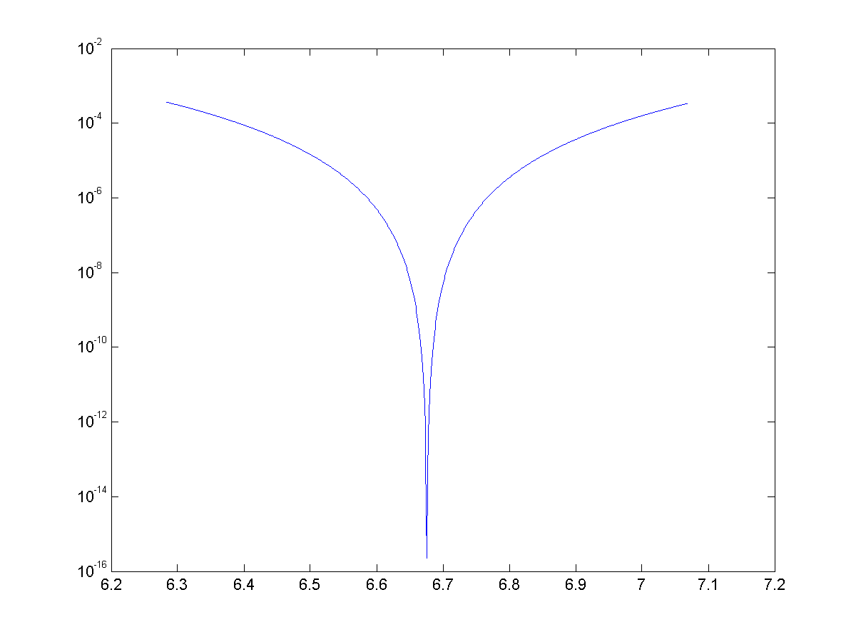
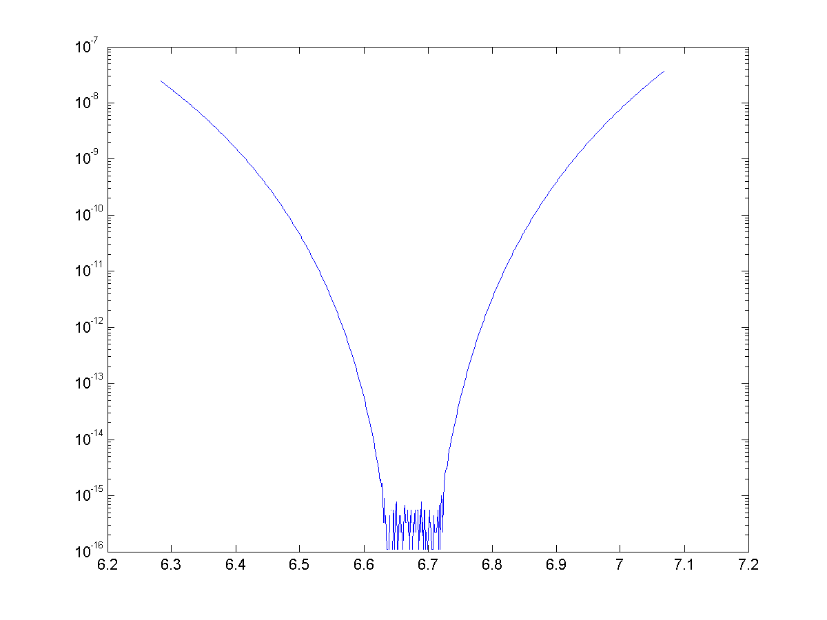
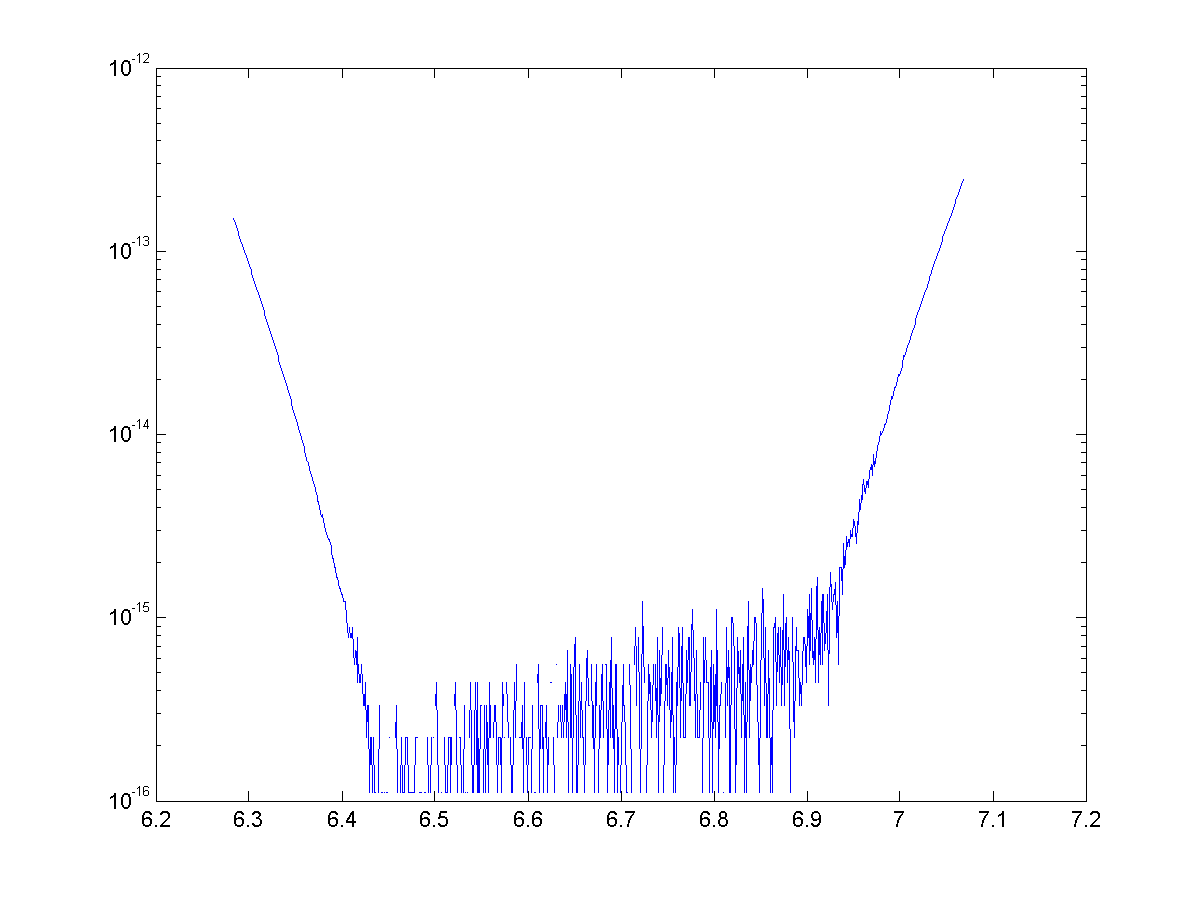
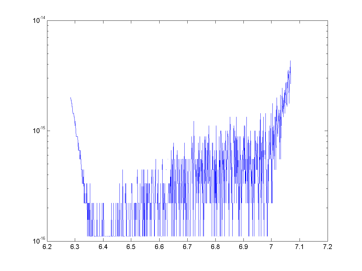
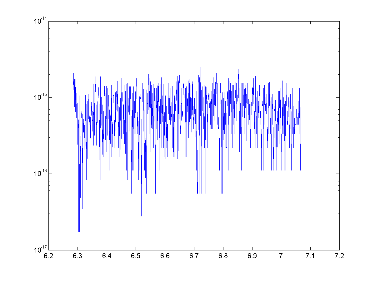
Once again we have generated some exciting looking, but nonetheless useless approximations. We were able to use binomial theorem and some trickery to generate approximations with great accuracy, but once again they are nowhere near as speedy to calculate as the Maclaurin series.
Representing Trigonometric Functions with the Binomial Series
Posted on April 4, 2014
In this post, we will introduce the incredibly useful binomial theorem and series, then use the series and De Moivre's theorem to derive a representation and approximations for trigonometric functions.
Background
The binomial theorem is a way to expand a binomial raised to a power. For a natural number $n \in \mathbb{N}$ the binomial theorem is $$ (a+b)^n={n \choose 0} a^n b^0 + {n \choose 1} a^{n-1}b+{n \choose 2} a^{n-2}b^2…+{n \choose n} a^0 b^{n}.$$
A tidier closed form expression is $$ (a+b)^n=\sum_{k=0}^{n}{ {n \choose k} a^{n-k}b^{k} } .$$ Closely related to the binomial theorem (integer exponents) is the binomial series (for non-integer exponents).
For a real exponent $\alpha \in \mathbb{R}$ the binomial theorem becomes: $$ (a+b)^{\alpha}=\sum_{k=0}^{\infty}{ {\alpha \choose k} a^{\alpha-k}b^{k} } .$$ Without getting too in depth on convergence, it is important that $a<b$. The convergence of this series when $a=b$ depends on $\alpha$. There is more on convergence here.
Even if $\alpha$ isn't an integer, the coefficients ${ \alpha \choose k}$ are calculated similarly. Let’s look at two examples.
For integers: $${ 7 \choose 3}=\frac{7\cdot 6\cdot 5}{3\cdot 2\cdot 1}=35.$$ For non-integers: $${ 7.2 \choose 3}=\frac{7.2\cdot 6.2\cdot 5.2}{3\cdot 2\cdot 1}=38.688.$$ The generalized binomial has some useful applications like approximating roots, deriving multiple angle formulas, and approximating $e$.
Deriving a series
The starting point for deriving these series is De Moivre's Theorem. The theorem is most commonly in used complex analysis, but it is probably best known as a tool for deriving multiple angle formulas. This theorem can be found in any complex analysis text, but we will state it here for clarity.
De Moivre's Theorem: For $n\in \mathbb{Z}$ and $\phi \in \mathbb{R}$
In multiple angle formula derivations, $n$ is generally a constant integer and $\phi$ is a variable. However, there are two significant differences in our approximations. We will leave $\phi$ constant and we will replace $n$ with a variable $\alpha \in \mathbb{R}$ that can vary.
In general, De Moivre's Theorem breaks down when generalized to $\alpha \in \mathbb{R}$. Any standard complex analysis book can provide examples of this. The proof is a little dry so we won’t show it here, but It can be shown that as long as we pick $\phi \in (-\pi,\pi]$, our generalization of De Moivre's Theorem holds.
Let $\phi \in (-\pi,\pi]$ with $\phi \neq 0$ and let $\theta=\alpha\phi$ for $\alpha \in \mathbb{R}$. Now we can take this special case of De Moivre's Theorem and apply the generalized binomial theorem, yielding: \begin{eqnarray*} \cos{\theta}+i\sin{\theta}&=&\cos{\alpha\phi}+i\sin{\alpha\phi}\\ &=&(\cos{\phi}+i\sin{\phi})^\alpha \\ &=&\displaystyle\sum_{k=0}^\infty{i^k{\alpha\choose k}\cos^{\alpha-k}{\phi}\sin^{k}{\phi} } \\ &=&\cos^{\alpha}{\phi}\displaystyle\sum_{k=0}^\infty{i^k{\alpha\choose k}\tan^{k}{\phi} }\\ &=&\cos^{\alpha}{\phi}\displaystyle\sum_{k=0}^\infty{(-1)^k\left[{\alpha\choose 2k}\tan^{2k}{\phi}+ i{\alpha \choose 2k+1}\tan^{2k}{\phi}\right]}. \end{eqnarray*} Now we equate the real and imaginary parts: \begin{eqnarray*} \cos{\theta}&=&\cos^{\alpha}{\phi}\displaystyle\sum_{k=0}^\infty{(-1)^k{\alpha\choose 2k}\tan^{2k}{\phi} } \\ \sin{\theta}&=&\cos^{\alpha}{\phi}\displaystyle\sum_{k=0}^\infty{(-1)^k{\alpha \choose 2k+1}\tan^{2k+1}{\phi} }. \end{eqnarray*} We can also create an alternative form by letting $x=\tan\phi \rightarrow \cos\phi=1/\sqrt{1+x^2}$: \begin{eqnarray*} \cos{\theta}&=&\left(1+x^2\right)^{-\alpha/2}\displaystyle\sum_{k=0}^\infty{(-1)^k{\alpha\choose 2k}x^{2k} } \\ \sin{\theta}&=&\left(1+x^2\right)^{-\alpha/2}\displaystyle\sum_{k=0}^\infty{(-1)^k{\alpha \choose 2k+1}x^{2k+1} }. \end{eqnarray*} While we will not go in depth here, it is important to study the convergence of these series. As a general rule, the series will converge for $\phi$ such that $\cos{\phi}>\sin{\phi}$ (this can be verified with the ratio test). It can also be shown with the alternating series test that if $\cos{\phi}=\sin{\phi}$, then the series will converge for $\theta\geq-\pi/4$. Both series converge for the values of $\theta$ and $\phi$ chosen later in this paper.
Approximations
To implement these series as approximations, they must be truncated. The error associated with this truncation is heavily dependent on both $n$, the number of terms in the truncated series, and the value of $\phi$. The number of terms will be predetermined for consistency and computational efficiency. Realistically, values around $n=8$ are a good starting place because the standard approximation for trigonometric functions in MATLAB utilizes a truncated and slightly modified Maclaurin series with $8$ terms.
For the approximations to be repeatable without re-evaluating $\tan{\phi}$ and $\cos{\phi}$, the value of $\phi$ must be constant. With $\phi$ and $n$ constant, $\alpha$ will be recomputed for each $\theta$. Sensitivity studies on $\phi$ showed that approximations with $\tan{\phi}=.1$ are exceptionally accurate for a small number of terms, so that value will be used for approximations throughout the rest of the paper. Let’s try an example.
Example: Approximate $\cos{\pi/3}$.
Solution:Let $\phi=\tan^{-1}({.1})\approx.0997$. Then we compute $\alpha = \frac{\pi/3}{.0997} = 10.5.$ We will use $n=8$ terms in our approximation. We have \begin{eqnarray*} \cos{\pi/3} &\approx& \cos^{10.5}({.0997}) \displaystyle\sum_{k=0}^7{(-1)^k{10.5 \choose 2k}\tan^{2k}({.0997})} \\ &=&\cos^{10.5}({.0997}) \left[ 1-\frac{10.5(10.5-1)}{2!}.1^2+-... \ +-\frac{10.5(10.5-1)...(10.5-13)}{14!}.1^{14} \right] \\ &=&0.49999999999999944.\\ \end{eqnarray*} These approximations cannot be easily evaluated by hand, but can be carried out with a computer quickly and with exceptional accuracy. The outline and basic code for the cosine approximation are below.
- Specify $\phi$ and $n$
- Compute $\alpha$
- Initialize coefficient and sum variables
- Use an iterative loop to calculate the generalized binomial coefficients and new terms
- Multiply the sum by $\cos^\alpha(\phi)$
An example of this code is (written for MATLAB) is
[approx, error] = function calculate_theta(theta)
tan_phi=.1;
phi=0.099668652491162;
cos_phi=0.995037190209989;
alpha=theta/phi;

coeff=1;
n=8;
sum=0;

for i=1:n
    sum=sum+coeff;
    coeff=-tan_phi^2*coeff*(alpha-2*i+1)*(alpha-2*i+2)/(2*i)/(2*i-1);
end

approx=sum*cos_phi^alpha;
error=approx-cos(theta);
Recall, $\phi$ is predetermined, so $\tan{\phi}$ and $\cos{\phi}$ are constants. In this code, they are represented with tan_phi and cos_phi respectively. Also, theta represents $\theta$, alpha represents $\alpha$, n represents the number of terms in the truncated series, coeff is each term in the series, and sum is utilized in the loop to add up the terms.
Before we get too ahead of ourselves, we need to consider how this stacks up against existing approximations for trigonometric functions. The simplest is the Maclaurin Series, with example source code shown here. While our approximations are a novel new look, they take much longer to compute so they are not a viable replacement for any existing approximations.
Implicit finite difference formulation on an unstructured mesh
Posted on March 17, 2014
Introduction
Objective: Obtain a numerical solution for the 2D Heat Equation using an implicit finite difference formulation on an unstructured mesh in MATLAB. The temperature distribution over time for an example problem described below will look something like this:
Helpful background: basic understanding of PDEs (partial differential equations), basic MATLAB coding (for loops, arrays and structure arrays), and solution methods for matrix equations.
Modeling the physics
First let’s introduce the heat equation. The heat equation in two dimensions is $$u_t=\alpha(u_{xx}+u_{yy})$$ where $u(x,y,t)$ is a function describing temperature and $\alpha$ is thermal diffusivity.
Numerically discretizing the equations We are going to solve the heat equation numerically with finite differences on an unstructured mesh. This is a fairly non-standard approach; when numerical analysts encounter difficult geometries they typically move on from cartesian finite difference for coordinate transformations, or other methods like finite volumes or finite elements on unstructured meshes.
We will keep as close as possible to the true nature of finite difference without using coordinate transformations. Our previous post did this as well, but what makes this method more desirable is the flexibility that comes from unstructured meshing. With an unstructured mesh, it is easier to mesh around complex geometries and add local refinement.
Approximating derivatives To create discretized equations we will need approximations for the second derivatives $u_{xx}$ and $u_{yy}$. We will go back to a Taylor series expansion, but this time extend it in in two dimensions. Consider a function $u$ at points $u_0=u(x_0,y_0)$ and $u_1=u(x_1,y_1)$ with $x_1=x_0+\Delta x$ and $y_1=y_0+\Delta y$. Then the two dimensional Taylor series expansion is $$ u_1 \approx u_0 + u_x\Delta x +u_y\Delta y +u_{xx}\Delta x^2 +u_{yy}\Delta y^2 +u_{xy}\Delta x \Delta y $$ We will treat $\Delta x$, $\Delta y$, $\Delta x^2$, $\Delta y^2$, $\Delta x\Delta y$, as coefficients and let the derivatives be the unknowns. Then we have a linear equation with five unknowns, $u_x$, $u_y$, $u_{xx}$, $u_{yy}$, and $u_{xy}$. That means to solve for all first and second derivatives requires five linearly independent equations, which we can get if we have $n \geq 5$ neighboring points that aren't collinear in the same direction.
Set it up as $A\textbf{x}=\textbf{b}$ where \[ \textbf{b} = \left[ \begin{array}{c} u_1-u_0 \\ u_2-u_0 \\ … \\ u_n-u_0 \end{array} \right] \] \[ \textbf{x} = \left[ \begin{array}{c} u_x \\ u_y \\ u_{xx} \\ u_{yy} \\ u_{xy} \\ \end{array} \right] \]
and $A$ is the coefficient matrix.
As one might guess, this results in approximations with second order accuracy for the first derivatives but only first order accuracy for the second derivatives, which is not acceptable accuracy. There are different ways to address this but the simplest is to add the third derivative terms to our equations. There are four third derivatives $u_{xxx}$, $u_{yyy}$, $u_{xxy}$, and $u_{xyy}$. This means we will need to use information from nine neighboring points to attain second order accuracy.
Now you may be wondering, how will we pick the nine neighboring points that best solve the physical problem? To best capture the physics we want equal weight from the surrounding points. However, unstructured meshes have a varying number of neighboring points, and often times have less than nine. To address this problem we will get greedy - we will not take just all neighboring points, but all the neighbors of neighboring points. This will leave us with much more than nine equations (generally 20-30) for only nine unknowns.
To best solve the overdetermined system we will use the least squares method. For an overdetermined system $A\textbf{x}=\textbf{b}$ the least squares solution is $$ \textbf{x}=\left[ (A^TA)^{-1}A^T \right] \textbf{b}$$ Let $\textbf{d}$ be the sum of the fourth and fifth rows of $(A^TA)^{-1}A^T$. Then we can write $$ (u_{xx}+u_{yy})_{x_0,y_0} = \textbf{d}\textbf{b}.$$ Since the mesh does not move we can use the same coefficients to calculate derivatives at every time step. Therefore these least squares calculations and assembly $\textbf{d}$ vectors (one for each node) of only need to be carried out once.
As we will show later in the code it is not good if the matrix has linearly dependent rows. To avoid this one could add an error check that eliminates $\Delta x$ and $\Delta y$ pairs that have close to the same angle. The closer points are to being linearly independent, the worse the condition of the matrix $A$. That said, if the angles differ by $180^{\circ}$ then rows are still linearly independent due to the nature of the coefficients.
Now that we have a way to calculate the derivatives, we can implement a formulation. We have shown the explicit FTCS formulation in two previous posts, so in this post we will just focus on an implicit method. We will use the Crank-Nicolson method (for more, check this paper on finite differences with the heat equation).
Implicit formulation (Crank-Nicolson)
The approximation becomes \begin{eqnarray} u_t^n &=& \alpha\cdot(u_{xx}+u_{yy}) \\ \frac{u^{n+1}-u^n}{dt} &=& \frac{\alpha}{2} \left[ (u_{xx}+u_{yy})^{n+1} + (u_{xx}+u_{yy})^n \right] \\ u^{n+1} - \frac{\alpha\cdot dt}{2}(u_{xx}+u_{yy})^{n+1} &=& u^n + \frac{\alpha\cdot dt}{2}(u_{xx}+u_{yy})^n \\ u^{n+1} - \frac{\alpha\cdot dt}{2} \textbf{d}\textbf{b}^{n+1} &=& u^n + \frac{\alpha\cdot dt}{2} \textbf{d}\textbf{b}^n \end{eqnarray} The left hand side of the equation is called the implicit side and contains the unknowns $u^{n+1}$ and $\textbf{b}^{n+1}$. The right hand side is all known values ($u^n$ and $\textbf{b}^n$ are from the previous time step) and is called the explicit side.
If we create an equation like this for each of the $n$ point in our domain then we have a system of $n$ equations with $n$ unknowns in the form $A\textbf{x}=\textbf{b}$ where $\textbf{x}$ is all of the $u^{n+1}$ values, $\textbf{b}$ is the explicit side, and $A$ is the coefficients from the left hand side.
Example problem
For example we will use the same physical problem as in part 2 (the only difference is the length scale). A $1x1$ flat plate has a thermal diffusivity of $\alpha=.001$. The temperature is fixed at $u=1$ on an inner circular boundary and is fixed at 0 on four outer boundaries. Elsewhere, the initial temperature is $u=0$. Find the temperature distribution over time.
Meshing
Much of the best meshing software is propietary and expensive, but there are some good free programs like Gmsh. We will implement code to read in and use a *.msh file.
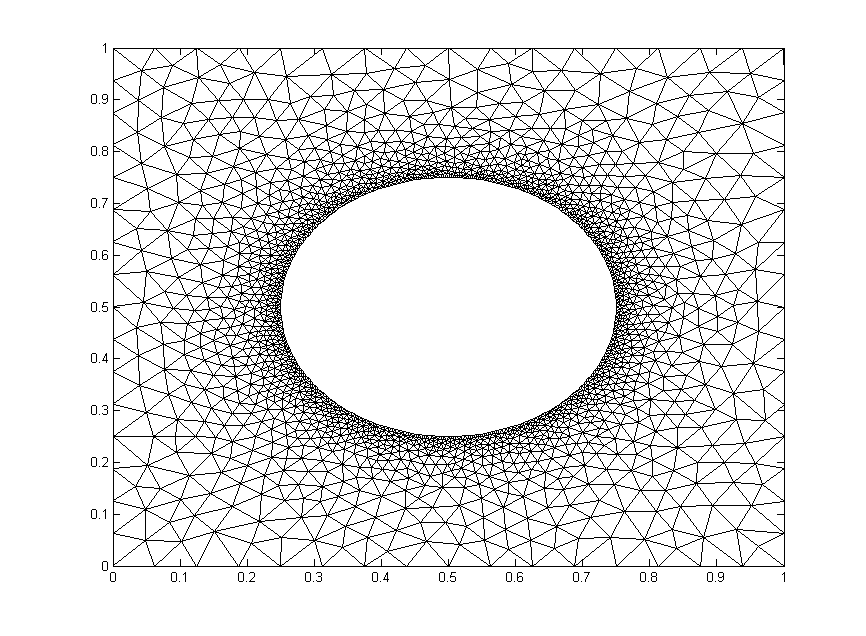
We will test out the mesh below. It has $1,992$ nodes.
The code
Now let’s lay out the code. We are going to break it up into three steps: initialize relevant physical parameters, import the mesh, set the boundary conditions, assemble the coefficient matrix, and set up the time loop.
Step 1: Initialize physical parameters
%Physical Quantities
nts=100; ntsabout=100;
dt=.03; alpha=.001; c=alpha*dt/2;
Step 2: Import the Mesh
[xyz,mesh,nn,tri,bnd,map]=importmesh2('circle_fine.msh');
The function will return
- xyz: the nodes in a (nn,2) where nn is the number of points in the mesh.
- mesh: A structure array containing the fields nbr (neighboring points), dx and dy (the distances to respective points), coeff the coefficients of the derivative approximation, and bnd, the boundary type of the point.
- tri: the “connectivity of the mesh (for visualizations).
- nn: The number of nodes in the mesh
- bnd: a list of the nodes in the boundary. Only necessary for an implicit formulation.
- map: The points in the mesh not on a boundary.
I will not include the importmesh2 code in this post but you can access the text here.
Step 3: Apply Initial and Boundary Conditions
%Initialize arrays
T = zeros(nn,1); A=zeros(nn); b=zeros(nn,1);

%Initial conditions
for n=bnd
    if mesh(n).bnd==5
        T(n)=1;
    end
end
Step 4: Assemble coefficient matrix and boundary contribution to the rhs vector
for i=bnd
    A(i,i)=1;
end

for i=map
    A(i,i)=1+c*mesh(i).coeff(end);
    for j = 1:length(mesh(i).nbr)
        A(i,mesh(i).nbr(j))= -c*mesh(i).coeff(j);
    end
end

b(bnd)=T(bnd);
Step 5: Time Loop
for t=1:nts
    %update rhs
    for n=map
        dd=mesh(n).coeff*[T(mesh(n).nbr); -T(n)];
        b(n)=c*dd+T(n);
    end

    %solve matrix equation
    %T=Ai*b;             %use inverse of A, requires Ai=inv(A)
    %T=A\b;              %MATLAB built in mldivide
    %T=L\T; %T=U\T;      %LU decomposition, requires [L,U]=lu(A);
    [T,flag]=gmres(A,b); %GMRES method

    %update visualization
    if mod(t,ntsabout)==0
        trisurf(tri,xyz(:,1),xyz(:,2),T,'FaceColor','interp','EdgeColor', 'none')
        axis([0,1,0,1]); view(0,90); colorbar; grid off;
        outframe(t) = getframe;
    end
end %time loop
Results
We already showed a visualization at the top of the post so let's look at run-time comparison of explicit and a few different matrix solver methods with implicit. The methods are explicit (FTCS), MATLAB’s mldivide (\), $LU$ decomposition with back-substitution, inverting $A$, and the GMRES method. We used the mesh shown above and a refined mesh with four times as many nodes. We calculated two time lengths, $3~\mathrm{s}$ and $30~\mathrm{s}$. Computation times are given in seconds.
| Method | $t=3~\mathrm{s}$ (coarse) | $t=30~\mathrm{s}$ (coarse) | $t=3~\mathrm{s}$ (fine) | $t=30~\mathrm{s}$ (fine) |
|---|---|---|---|---|
| Explicit | 11.94 | 121.30 | N/a | N/a |
| A\b | 42.28 | 411.5 | N/a | N/a |
| LU | 2.50 | 25.04 | 35.35 | 184.5 |
| Inversion | 1.72 | 17.08 | 67.42 | 146.8 |
| GMRES | 2.76 | 24.18 | 29.71 | 225.3 |
Since the coefficient matrix doesn’t change with every time step, the speed during the time loop is greatly increased by inverting $A$ or determining its $LU$ decomposition beforehand. The GMRES method on the other hand, is fast because it is designed to handle sparse matrices like $A$.
We are only able to get away with inverting $A$ because our mesh is very small. Matrix inversion is a computationally expensive operation that does not scale well (see here). For example, if one quadruples the mesh points as we have, the run time for inverting $A$ theoretically increases by a factor of 64. Furthermore MATLAB documentation recommends against using the inv command whenever possible. The $LU$ decomposition is generally considered to be better practice than inversion, but it also scales poorly for large matrices unless an algorithm that takes advantage of the sparse nature of $A$ is employed.
In a reasonably large computation, GMRES would generally be the best method unless another method can be employed that efficiently inverts sparse matrices (such methods exist for specialized problems).
Structured, transformation-free finite differences on complex geometries
Posted on January 22, 2014
Introduction
Objective: Obtain a numerical solution for the 2D Heat Equation on mesh with circular boundaries in MATLAB using an explicit finite difference formulation with Richardson extrapolation (and without coordinate transformation).
Helpful background: A basic understanding of PDEs (partial differential equations), MATLAB coding (for loops, arrays, functions, maps, trisurf, and bitget), basic derivative approximations with finite differences and Richardson extrapolation.
Modeling the problem
First let’s introduce the heat equation. The heat equation in two dimensions is $$u_t=\alpha(u_{xx}+u_{yy})$$ where $u(x,y,t)$ is a function describing temperature and $\alpha$ is thermal diffusivity.
Numerically discretizing the equations We are going to solve the heat equation numerically with an explicit formulation. We talk about this a little in our previous post on the heat equation. There are many methods that solve this, but the simplest is an explicit finite difference formulation. The major difference here is how we handle the more difficult geometry of a circular disk. If none of the points neighbor the boundary, we will use the central difference approximation for our second derivatives. The approximations for $u_{xx}$ and $u_{yy}$ are \begin{eqnarray} u_{xx}(i,j)=\displaystyle\frac{u(i+1,j)-2\cdot u(i,j)+u(i-1,j)}{(\Delta x)^2} \\ u_{yy}(i,j)=\displaystyle\frac{u(i,j+1)-2\cdot u(i,j)+u(i,j-1)}{(\Delta y)^2}. \end{eqnarray}
Calculating the second derivatives for points near boundaries with curvature will be covered in the next two sections.
We will then update the temperature using a first derivative forwards in time. $$ u_t^n=\frac{u^{n+1}-u^n}{\Delta t}.$$ The final formulation is then \begin{eqnarray} u^{n+1}(i,j) &=& u^n(i,j)+\alpha\cdot \Delta t\cdot \left(u_{xx}^n(i,j)+u_{yy}^n(i,j)\right) \end{eqnarray}
Geometries with Curvature When geometries become more complex than a 1D problem on a line or a 2D cartesian grid, many numerical analysts move on to one of three methods: finite volume methods, finite element methods, or finite difference methods with coordinate transformations. These formulations are much more difficult to implement, but can essentially handle any geometry (with varying difficulty).
Instead of using one of these methods we will stick with finite differences and take advantage of a tool call Richardson extrapolation to keep the second order accuracy that led to a nice solution in Part 1.
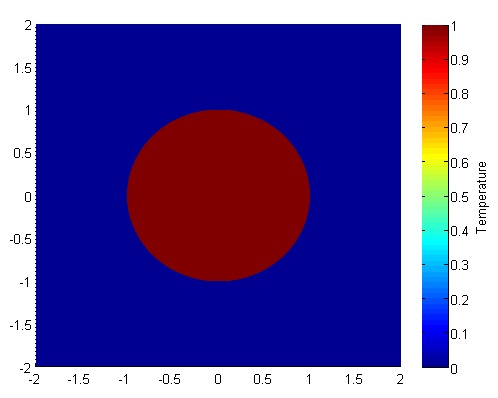
Let’s set up a specific example. A $4x4$ flat plate has a thermal diffusivity of $\alpha=.01$. The temperature is fixed at $u=1$ in an inner circle with radius $1$. Elsewhere, the initial temperature is $u=0$ and the outer boundaries are fixed at $u=0$ for all time. Find the temperature distribution over time.
(Note: I left off any units and have some simplified numbers for temperature and plate dimensions. Feel free to change them as you please, but make sure your formulation is still stable.)
The initial condition would look something like this:
Richardson Extrapolation Before we get started, it may help to glance at some of the basics of Richardson Extrapolation at Wikipedia.
The biggest challenge in our problem is that it requires a second derivative, which proves to be a little harder to compute with second order spatial accuracy. First and foremost, we can’t do it with just the two neighboring points (like we would be able to with evenly spaced points); we will need to use one more. Consider the points below. Assume that at each point $1,2,3,4$ we know the value of a function $f$ are $f_1,f_2,f_3,f_4$.
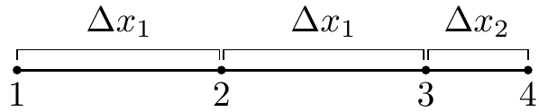
We will use information at the points $1,2,3,$ and $4$ to approximate the second derivative at point $3$, $f_3^{\prime\prime}$ . Why point $3$? In our particular problem, the second derivatives at points $1$ and $2$ can be approximated with a standard central difference and point $4$ will be a boundary, so the second derivative will not need to be calculated there.
Our first step will be to calculate the first derivatives at points $2,3,$ and $4$. These are fairly straightforward; we will use a central difference at point $2$ and Richardson extrapolation and points 3 and 4. They should look something like this \begin{eqnarray} f_2^{\prime} &=& \displaystyle\frac{f_3-f_1}{2\cdot \Delta x_1} \\ f_3^{\prime} &=& \displaystyle\frac{k_1\cdot (f_4-f_3)}{(k_1+1)\cdot \Delta x_2}+\frac{(f_3-f_2)}{(k_1+1)\cdot\Delta x_1} \\ f_4^{\prime} &=& \displaystyle\frac{k_2\cdot (f_4-f_3)}{(k_2-1)\cdot\Delta x_2}-\frac{f_4-f_2}{(k_2-1)\cdot (\Delta x_1+\Delta x_2) } \end{eqnarray} Where $k_1= \frac{ \Delta x_1}{ \Delta x_2}$ and $k_2=\frac{ \Delta x_1+ \Delta x_2}{ \Delta x_2}$ . Now we will use these to approximate the second derivative at $x_3$ with Richardson extrapolation. This is very similar to the formula except we will use a different value of $k$, namely $k_3=\frac{4\cdot k_1-1}{2\cdot k_1-2}$.
After wading through the algebra, your expression will simplify to $$f_3^{\prime\prime} = \frac{\Delta x_2^3\cdot (f_1-2 f_2+f_3)+\Delta x_1^3\cdot (6 f_4-6 f_3)+\Delta x_1^2\cdot \Delta x_2\cdot (-f_1+8 f_2-7 f_3)}{\Delta x_1^2\cdot \Delta x_2\cdot (\Delta x_1+\Delta x_2)\cdot (2 \Delta x_1+\Delta x_2)} $$
This is a pretty costly formula compared to the central difference method. Fortunately, we will not have to use this equation very often; only when the points are neighboring the boundary. Meanwhile, this allows us to use the cheap and effective central difference method at all other points. Therefore the overall computation should be fairly inexpensive.
We will also need to generate a mesh. Below is an example of the mesh. The elements have been triangulated for simple viewing in MATLAB, but there is no triangulation and no element formulation in the solution.
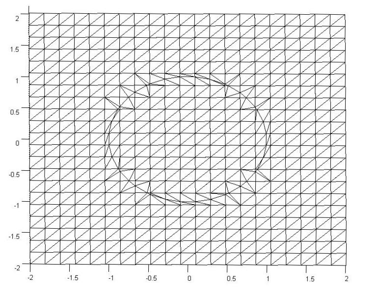
The original mesh here was a $22x22$ grid, but there were an additional 40 points added on the boundary to maintain the curvature of the circle. The important part is finding the $\Delta x_2$ and $\Delta y_2$ values for each of the points immediately neighboring a boundary and creating an additional point on the mesh.
When we loop through the mesh points we will ignore all points where the temperature is specified, use Richardson Extrapolation on the points adjacent to the 40 added points, and uses central differences elsewhere.
A Quick Look at Stability In the previous part we discussed stability, namely that in order for the old formulation to hold we needed to satisfy $$ \Delta t < \frac{\Delta x_1^2}{4\alpha}.$$ We will not perform a proper stability analysis, but our empirical results show that $$ \Delta t < \frac{\Delta x_1\cdot min(\Delta x_2)}{4\alpha}$$ is generally sufficient. Once you have your code written it is easy to empirically test different values of $\Delta t$.
The code
We are going to break it up into five steps: Create the Richardson extrapolation function, initialize relevant physical values, generate the mesh, set the boundary conditions, and set up the time loop. The time loop will consist of calculating the derivatives at each point, updating the temperature for each point, and then updating the visualization.
Step 1 Richardson Extrapolation
function [ddf3a] = richardson(dx1,dx2,f1,f2,f3,f4)
ddf3a = (dx2^3*(f1-2*f2+f3) + ...
         dx1^3*(6*f4-6*f3) + ...
         dx1^2*dx2*(-f1+8*f2-7*f3))...
       /(dx1^2*dx2*(dx1+dx2)*(2*dx1+dx2));
end
Step 2 Initialize variables
%Initialize Physical Values
dt=.01;                     %time step
nts=500;                    %number of time steps
alpha=.01;                  %thermal diffusivity
bounds=[-2 2 -2 2];         %corners of outer domain

%Mesh Variables
nx=50; ny=50;               %number of points in the x and y directions
%distance in between points
dx1=(bounds(2)-bounds(1))/(nx-1);
dy1=(bounds(4)-bounds(3))/(ny-1);
Step 3 Generate the Mesh
[xyz,skip,dx2,dy2,tri]=genmesh(bounds,nx,ny);

%The derivatives and temperature will be stored in a 1D arrays
nodes=length(skip);
uxx=zeros(nodes,1); uyy=zeros(nodes,1); T=zeros(nodes,1);
The function will return
- xyz: the nodes in a (np,2) where np is the number of points in the mesh.
- skip: an array that shows whether a point is on a boundary or neighboring one.
- dx2 and dy2: maps relating the distance from a point to the boundary if it neighbors the boundary.
- tri the “connectivity" of the mesh.
An alternative to creating your own tri connectivity would be using the MATLAB built in function tri=delaunay(x,y) but it will not look as good as if you make it yourself.
I will not include any of the code in this post (my version is 160 lines long and it is mostly boring) but you can access the text here.
Step 4 Apply Initial and Boundary Conditions
for p=1:length(skip)
    if skip(p) < 0
        u(p)=1.0;
    else
        u(p)=0.0;
    end
end
Step 5 Time Loop The time loops has three components, first calculate the second derivatives, then update temperature, then update the visualization.
One note before we get into the code. We are using the MATLAB function “bitget” which determines based of the values of skip(p) (see Step 3) whether it is close to the boundary. This is by all means not necessarily the best way to determine whether a point neighbors a boundary, but it works and is not too costly.
for t=1:nts
    for i=2:ny-1
        for j=2:nx-1
            p=nx*(i-1)+j;
            if skip(p) < 0
                continue
            end
            if     bitget(skip(p),1)==1
                uxx(p)=richardson(dx1,abs(dx2(p)),u(p-2),u(p-1),u(p),T_b);
            elseif bitget(skip(p),3)==1
                uxx(p)=richardson(dx1,abs(dx2(p)),u(p+2),u(p+1),u(p),T_b);
            else
                uxx(p)=(u(p-1)-2*u(p)+u(p+1))/dx1^2;
            end

            if     bitget(skip(p),2)==1
                uyy(p)=richardson(dy1,abs(dy2(p)),u(p-2*nx),u(p-nx),u(p),T_b);
            elseif bitget(skip(p),4)==1
                uyy(p)=richardson(dy1,abs(dy2(p)),u(p+2*nx),u(p+nx),u(p),T_b);
            else
                uyy(p)=(u(p-nx)-2*u(p)+u(p+nx))/dy1^2;
            end
        end
    end

    for i=2:nx-1
        for j=2:ny-1
            p=nx*(i-1)+j;
            if skip(p)<0
                continue
            end
            u(p)=u(p)+alpha*dt*(uxx(p)+uyy(p));
        end
    end
    trisurf(tri,xyz(:,1),xyz(:,2),u,'FaceColor','interp');
    frame = getframe(1);
end
Results
Below are two animations of the temperature distribution over time.
Some notes about the code
If you are a novice programmer, you may not have heard of maps. Maps are "objects with keys that index to values" (see here and here). They are similar to an array, except that keys must be unique, keys don't need to be integers, and key values typically aren't ordered. A map is by no means necessary here, but it is an efficient way to store and quickly retrieve the $\Delta x_2$ and $\Delta y_2$ values.
The most confusing part of the code above is implementation of the skip array with bitget. Basically, skip is an array with an integer for every node.
- If a node p is on or inside the circle, skip(p)=-1.
- If it is outside the circle and not adjacent to it, skip(p)=0.
- If it is adjacent to the circle (left, below, right, above) then we add 1,2,4,8 respectively to skip(p). For example, if a point is below and to the right of points on the circle, then skip(p)=6.
We can then reverse engineer skip(p) with bitget. This is not necessarily the best or only way, but it is a relatively simple implementation.
You can save some space in memory by letting uxx and uyy be single values instead of arrays. This however, would either require two arrays for temperature (an old and a new) or some algorithm to keep from overwriting old values of temperature before all derivatives are calculated. Since we are dealing with a relatively coarse 2D mesh, this is not a significant issue.
Finite Difference Solution of the Heat Equation on a Structured Mesh
Posted on November 19, 2013
Introduction
In this post we will numerically solve the heat equation with an explicit finite difference formulation.
Objective: Obtain a numerical solution for the 2D Heat Equation in MATLAB using an explicit finite difference formulation.
Helpful background: basic understanding of PDEs (partial differential equations), basic MATLAB coding (for loops and arrays), and basic derivative approximations with finite differences.
Modeling the problem
First let’s introduce the heat equation. The heat equation in two dimensions is $$u_t=\alpha(u_{xx}+u_{yy})$$ where $u(x,y,t)$ is a function describing temperature and $\alpha$ is thermal diffusivity.
Numerically discretizing the equations We are going to solve the heat equation numerically. There are many methods that solve this, but the simplest is an explicit finite difference formulation. Explicit means the solution at a certain time step depends only on previous step, as opposed to implicit (see here) where the solution depends on next time step. Finite differences are a simple way to use neighboring grid points to approximate derivatives.
We will use the central difference approximation for our second derivatives. The approximations for $u_{xx}$ and $u_{yy}$ are \begin{eqnarray} u_{xx}(i,j)&=&\displaystyle\frac{u(i+1,j)-2\cdot u(i,j)+u(i-1,j)}{(\Delta x)^2} \\ u_{yy}(i,j)&=&\displaystyle\frac{u(i,j+1)-2\cdot u(i,j)+u(i,j-1)}{(\Delta y)^2}. \end{eqnarray} These are all at time $n$ (they are not exponents). We will use the forward difference approximation for $u_t$. We have
$$ u_t^n=\frac{u^{n+1}-u^n}{\Delta t}.$$
This is for every point $(i,j)$. Now we can take these 3 expressions, combine them, and solve for $u^{n+1}$.
\begin{eqnarray} u_t^n(i,j) &=& \alpha(u_{xx}^n(i,j)+u_{yy}^n(i,j)) \\ \frac{u^{n+1}(i,j)-u^n(i,j)}{\Delta t} &=& \alpha\left[\frac{u(i+1,j)-2\cdot u(i,j)+u(i-1,j)}{(\Delta x)^2}+ \frac{u(i,j+1)-2\cdot u(i,j)+u(i,j-1)}{(\Delta y)^2}\right] \\ u^{n+1}(i,j) &=& u^n(i,j)+\alpha\cdot dt\left[ \frac{u(i+1,j)-2\cdot u(i,j)+u(i-1,j)}{(\Delta x)^2}+\frac{(u(i,j+1)-2\cdot u(i,j)+u(i,j-1)}{(\Delta y)^2}\right] \end{eqnarray}
A quick look at stability The formulation we used (forward in time, centered in space) is only conditionally stable. We can show (but won’t here) with Von Neumann Stability Analysis, that we need the discretized time step $\Delta t$ to satisfy $$ \Delta t< \frac{\Delta x^2}{4\alpha}.$$Once you have your code written it is easy to empirically test this.
The code
Let’s set up a specific example. A $1x1$ flat plate has a thermal diffusivity of $\alpha=.01$. The temperature is fixed at $u=1$ on the top and right edges and $u=0$ on the bottom and left edges. Elsewhere, the initial temperature is $u=0$. Find the temperature distribution over time.
(Note: I left off any units and have some simplified numbers for temperature and plate dimensions. Feel free to change them as you please, but make sure your formulation is still stable.)
Now let’s lay out the code. We are going to break it up into three steps: Initialize relevant physical values, set the boundary conditions, and set up the time loop. The time loop will consist of calculating the derivatives at each point, updating the temperature for each point, and then updating the visualization.
Step 1: Initialize variables We will start by initializing relevant physics variables for the time step size, number of time steps, thermal diffusivity, reference plate length, number of points in the x and y direction, and the spatial discretization $\Delta x$ and $\Delta y$.
You can also preallocate the matrices for $u$, $u_{xx}$, and $u_{yy}$.
%Initialize Variables
dt=.005;                   %time step
nts=500;                   %number of time steps
alpha=.01;                 %thermal diffusivity
l=1;                       %reference length plate
nx=50; ny=50;              %number of points in the x and y directions
dx=l/(nx-1); dy=l/(ny-1);  %discretized distance in between points

%Temperature and the derivatives will be stored in a two dimensional array
u = zeros(nx,ny); uxx = zeros(nx,ny); uyy = zeros(nx,ny);
Step 2: Apply Initial and Boundary Conditions
%Initial/Boundary Conditions
for i=1:ny
   u(1,i)=1;
end

for i=1:nx-1
   u(i,ny)=1;
end
Step 3: Time Loop Here is the meat of the code. The time loops has three components, first calculate the second derivatives, then update temperature, then update the visualization.
for t=1:nts
   %Calc the Spatial 2nd Derivative, Centered in Space
   for i=2:nx-1
      for j=2:ny-1
         uxx(i,j)=(u(i+1,j)-2*u(i,j)+u(i-1,j))/(dx)^2;
         uyy(i,j)=(u(i,j+1)-2*u(i,j)+u(i,j-1))/(dy)^2;
      end
   end

   %Update Temperature, Forwards in Time
   for i=2:nx-1
      for j=2:ny-1
         u(i,j)=u(i,j)+alpha*(uxx(i,j)+uyy(i,j))*dt;
      end
   end

   %Visualization
   contourf(u)
   axis equal
   M(t) = getframe;
end %time loop
Results
Below are 2 GIFs (one is a contour plot, the other is a surface plot) of the temperature distribution over time.