Finite Difference Solution of the Heat Equation on a Structured Mesh
Posted on November 19, 2013
Introduction
In this post we will numerically solve the heat equation with an explicit finite difference formulation.
Objective: Obtain a numerical solution for the 2D Heat Equation in MATLAB using an explicit finite difference formulation.
Helpful background: basic understanding of PDEs (partial differential equations), basic MATLAB coding (for loops and arrays), and basic derivative approximations with finite differences.
Modeling the problem
First let’s introduce the heat equation. The heat equation in two dimensions is $$u_t=\alpha(u_{xx}+u_{yy})$$ where $u(x,y,t)$ is a function describing temperature and $\alpha$ is thermal diffusivity.
Numerically discretizing the equations We are going to solve the heat equation numerically. There are many methods that solve this, but the simplest is an explicit finite difference formulation. Explicit means the solution at a certain time step depends only on previous step, as opposed to implicit (see here) where the solution depends on next time step. Finite differences are a simple way to use neighboring grid points to approximate derivatives.
We will use the central difference approximation for our second derivatives. The approximations for $u_{xx}$ and $u_{yy}$ are \begin{eqnarray} u_{xx}(i,j)&=&\displaystyle\frac{u(i+1,j)-2\cdot u(i,j)+u(i-1,j)}{(\Delta x)^2} \\ u_{yy}(i,j)&=&\displaystyle\frac{u(i,j+1)-2\cdot u(i,j)+u(i,j-1)}{(\Delta y)^2}. \end{eqnarray} These are all at time $n$ (they are not exponents). We will use the forward difference approximation for $u_t$. We have
$$ u_t^n=\frac{u^{n+1}-u^n}{\Delta t}.$$
This is for every point $(i,j)$. Now we can take these 3 expressions, combine them, and solve for $u^{n+1}$.
\begin{eqnarray} u_t^n(i,j) &=& \alpha(u_{xx}^n(i,j)+u_{yy}^n(i,j)) \\ \frac{u^{n+1}(i,j)-u^n(i,j)}{\Delta t} &=& \alpha\left[\frac{u(i+1,j)-2\cdot u(i,j)+u(i-1,j)}{(\Delta x)^2}+ \frac{u(i,j+1)-2\cdot u(i,j)+u(i,j-1)}{(\Delta y)^2}\right] \\ u^{n+1}(i,j) &=& u^n(i,j)+\alpha\cdot dt\left[ \frac{u(i+1,j)-2\cdot u(i,j)+u(i-1,j)}{(\Delta x)^2}+\frac{(u(i,j+1)-2\cdot u(i,j)+u(i,j-1)}{(\Delta y)^2}\right] \end{eqnarray}
A quick look at stability The formulation we used (forward in time, centered in space) is only conditionally stable. We can show (but won’t here) with Von Neumann Stability Analysis, that we need the discretized time step $\Delta t$ to satisfy $$ \Delta t< \frac{\Delta x^2}{4\alpha}.$$Once you have your code written it is easy to empirically test this.
The code
Let’s set up a specific example. A $1x1$ flat plate has a thermal diffusivity of $\alpha=.01$. The temperature is fixed at $u=1$ on the top and right edges and $u=0$ on the bottom and left edges. Elsewhere, the initial temperature is $u=0$. Find the temperature distribution over time.
(Note: I left off any units and have some simplified numbers for temperature and plate dimensions. Feel free to change them as you please, but make sure your formulation is still stable.)
Now let’s lay out the code. We are going to break it up into three steps: Initialize relevant physical values, set the boundary conditions, and set up the time loop. The time loop will consist of calculating the derivatives at each point, updating the temperature for each point, and then updating the visualization.
Step 1: Initialize variables We will start by initializing relevant physics variables for the time step size, number of time steps, thermal diffusivity, reference plate length, number of points in the x and y direction, and the spatial discretization $\Delta x$ and $\Delta y$.
You can also preallocate the matrices for $u$, $u_{xx}$, and $u_{yy}$.
%Initialize Variables
dt=.005;                   %time step
nts=500;                   %number of time steps
alpha=.01;                 %thermal diffusivity
l=1;                       %reference length plate
nx=50; ny=50;              %number of points in the x and y directions
dx=l/(nx-1); dy=l/(ny-1);  %discretized distance in between points

%Temperature and the derivatives will be stored in a two dimensional array
u = zeros(nx,ny); uxx = zeros(nx,ny); uyy = zeros(nx,ny);
Step 2: Apply Initial and Boundary Conditions
%Initial/Boundary Conditions
for i=1:ny
   u(1,i)=1;
end

for i=1:nx-1
   u(i,ny)=1;
end
Step 3: Time Loop Here is the meat of the code. The time loops has three components, first calculate the second derivatives, then update temperature, then update the visualization.
for t=1:nts
   %Calc the Spatial 2nd Derivative, Centered in Space
   for i=2:nx-1
      for j=2:ny-1
         uxx(i,j)=(u(i+1,j)-2*u(i,j)+u(i-1,j))/(dx)^2;
         uyy(i,j)=(u(i,j+1)-2*u(i,j)+u(i,j-1))/(dy)^2;
      end
   end

   %Update Temperature, Forwards in Time
   for i=2:nx-1
      for j=2:ny-1
         u(i,j)=u(i,j)+alpha*(uxx(i,j)+uyy(i,j))*dt;
      end
   end

   %Visualization
   contourf(u)
   axis equal
   M(t) = getframe;
end %time loop
Results
Below are 2 GIFs (one is a contour plot, the other is a surface plot) of the temperature distribution over time.

Projectile Motion with (Quadratic) Drag
Posted on October 31, 2013
Projectile motion is discussed and worked out in nearly every college physics, calculus, and dynamics class, but examples always seem to neglect or over-simplify drag. In this post we will tackle an analytic solution that models drag for a falling object.
Let’s suppose we are dropping a ball from a height \(h_0\) with a velocity \(v_0\). In a vaccuum, the only force is gravity, $mg$. Then projectile motion without drag begins with Newton’s second law $$F_{net}=mg=ma \rightarrow a=g.$$ Acceleration can then be twice integrated with respect to time, yielding $$p(t)=\frac{g}{2}t^2+v_0t+h_0.$$ Given a constant force (i.e. not dependent on time or velocity) this is a simple integration with respect to time and the math is rather elementary. We can make it much more challenging by inserting an additional force term, drag, which is dependent on velocity: $$F=mg-D =ma \rightarrow a=g-D/m.$$ Many approximations for drag can be applied, but the most accurate model is $$D=1/2 \rho v^2\cdot c_d\cdot A.$$ Here \(c_d\) is coefficient of drag (dimensionless), A is the cross-sectional area, and \(\rho\) is the density of the medium the object is falling (e.g. air is $1.225 ~ \mathrm{kg}/\mathrm{m}^3$). Let’s jump into the math. $$a=g-D/m=g-\frac{\rho\cdot c_d\cdot A}{2m}v^2.$$ Now let \(a=dv/dt\) and for simplicity let \(k^2=\frac{\rho\cdot c_d\cdot A}{2mg}\). Coincidentally, $\frac{1}{k}$ is also the terminal velocity of a falling object. We have \begin{eqnarray} \frac{dv}{dt} &=& g-gk^2 v^2 \\ g\cdot dt &=& \frac{dv}{1-k^2 v^2}. \end{eqnarray} In its current form, this is not a simple integration. It can be evaluated with the hyperbolic arc-tangent, but to keep the equations in terms of more recognizable functions we will instead apply a partial fraction expansion $$\frac{dv}{1-k^2 v^2}=\frac{1}{2k}\left[\frac{dv}{v-1/k}-\frac{dv}{v+1/k}\right].$$
If this is confusing, you can review partial fraction expansions here
Now we can integrate \begin{eqnarray} g\cdot dt &=& \frac{1}{2k} \left[\frac{dv}{v+1/k}-\frac{dv}{v-1/k}\right]. \\ g\cdot t &=& \frac{1}{2k} \left[\ln(v+1/k)-\ln(v-1/k)\right]+C_1. \end{eqnarray}
We now have time as a function of velocity, but that isn’t very useful. Let’s see if we can solve for $v$: \begin{eqnarray} g\cdot t &=& \frac{1}{2k} \left[ \ln(v+1/k)-\ln(v-1/k) \right] +C_1 \\ g\cdot t &=& \frac{1}{2k}\cdot\ln\left[\frac{v+1/k}{v-1/k}\right]+C_1 \\ 2gk\cdot t+C_2 &=& \ln\left[\frac{v+1/k}{v-1/k}\right]\\ \end{eqnarray}
Now we can exponentiate both sides
\begin{eqnarray} Ce^{2gk\cdot t}=\frac{v+1/k}{v-1/k}=\frac{2/k}{v-1/k}+1. \\ \end{eqnarray} Now we can solve for $v$. \begin{eqnarray} v &=& \frac{2/k}{Ce^{2gk\cdot t}-1}+1/k. \\ &=& \frac{1}{k}\left(\frac{2}{Ce^{2gk\cdot t}-1}+1\right). \\ \end{eqnarray} Now we eliminate that pesky \(C\) by applying an initial condition for velocity. We are simply dropping something so let \(v(0)=0\).
We have \begin{eqnarray} v &=& \frac{1}{k}\left(\frac{2}{Ce^{2gk\cdot 0}-1}+1 \right) \\ &=& \frac{1}{k}\left(\frac{2}{C-1}+1 \right) \rightarrow C=-1. \end{eqnarray} Therefore $$v = \frac{1}{k}\left(1-\frac{2}{e^{2gk\cdot t}+1}\right).$$ Velocity is all fine and dandy, but what we are really after is position. This requires one more integration, but fortunately it’s a little simpler: This takes a little rewriting u-substitution. We have \begin{eqnarray} \frac{dp}{dt} &=& \frac{1}{k}\left(1-\frac{2}{e^{2gk\cdot t}+1}\right) \\ &=& \frac{1}{k}\left(1-\frac{2e^{2gk\cdot t}+2}{e^{2gk\cdot t}+1}+\frac{2e^{2gk\cdot t}}{e^{2gk\cdot t}+1}\right) \\ &=& \frac{1}{k}\left(1-2+\frac{2e^{2gk\cdot t}}{e^{2gk\cdot t}+1}\right). \end{eqnarray}
Now this is in a form where we can intuitively apply $u$-substitution. We have \begin{eqnarray} p=\frac{1}{gk^2}\ln[e^{2gk\cdot t}+1]-\frac{t}{k}+C. \end{eqnarray} Now if we apply the initial condition \(h(0)=h_0\) we have \begin{eqnarray} p &=& \frac{1}{gk^2} \ln\left[e^{2gk\cdot t}+1\right]-\frac{\ln(2)}{gk^2}-\frac{t}{k}+h_0. \\ &=& \frac{1}{gk^2} \ln\left[\frac{e^{2gk\cdot t}+1}{2}\right]-\frac{t}{k}+h_0. \end{eqnarray}
Let's put this to use with a quick example. Let's say we are dropping two balls off a tower $56~\mathrm{m}$ tower. They have the same cross-sectional area $A=1/3 ~ \mathrm{m}^2$ and drag coefficient $c_d=0.5$, but have different masses of $1 ~ \mathrm{kg}$ and $5 ~ \mathrm{kg}$. We can use the above formula to find how long it takes them to hit the ground.
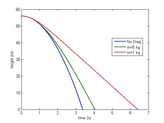
Clearly accounting for drag is important if the object falling is very light, very large, or is falling through a medium with a high density.