More Approximations for Trigonometric Functions with the Binomial Series
Posted on August 31, 2015
In this post, we will create a new set of approximations for sine and cosine that utilize the binomial series. Before you go any further, you may want to read this previous post where we walk through the binomial series and comparisons to the Maclaurin series.
Derivation
We are going to exploit Euler's formula with a twist. To refresh your memory, here's Euler's Formula. \begin{equation} \cos(\theta)+i\sin(\theta)=e^{i\theta} \end{equation} Now let's employ one of the older tricks in the book, adding and subtracting one from the same expression: \begin{equation} \cos(\theta)+i\sin(\theta)=\left[(e-1)+1\right]^{i\theta}. \end{equation} Now we have a binomial raised to a power. Once again, we will use known values and the binomial series to generate approximations for sine and cosine.
Fine Tuning For Approximation
In its current form this would almost be enough for decent approximations. However, closely tied to the accuracy of an approximation is the convergence rate of the series. To improve convergence, we want to make one of the terms small relative to the other term. Is there anything we can do here?
As a matter of fact, yes. We will employ a second manipulation - multiplying and dividing by the same number (inside and outside of the parentheses). Consider the updated equation \begin{equation} \cos(\theta)+i\sin(\theta)=a^i\cdot\left[\left(\displaystyle\frac{e}{a^{1/\theta}}-1\right)+1\right]^{i\theta}. \end{equation} If you need to, convince yourself that this is still valid. Now, to build a valid approximation, we need $\displaystyle\frac{e}{a^{1/\theta}}-1$ to be small for a range of values. In our previous post, we determined that you need a range of $\pi/4$ for sine and cosine, which could be extrapolated out to encompass all values.
Ideally we would just pick the range $[0,\pi/4]$, with which a value of $a=e^{\pi/8}$ would be a good place to center the approximation. However, If $\theta=0$, the expression \begin{equation} {(e^{\pi/8})^{1/0}}-1 \end{equation} is not defined (although the limit appears to exist).
On the other side of the range, at $\theta=\pi/4$, the expression becomes \begin{equation} \displaystyle\frac{e}{(e^{\pi/8})^{4/\pi}}-1=e^{1/2}-1\approx.64 \end{equation} which is enough for convergence, but maybe not optimal.
On the other hand, if we made the range $[2\pi,2\pi+\pi/4]$ with $a=2\pi+\pi/8$, then our bounding values are roughly $\approx\pm.06$ which will give us much better convergence. Due to the nature of this equation, rapidly increasing our range - for example, the range $[100\pi,100\pi+\pi/4]$ - has rapidly diminishing gains, and improved convergence will be offset by roundoff error elsewhere.
Implementing Approximations
An example of this code is (written for MATLAB) is
iterations=14;
start=2*pi;
range=pi/4;
increment=.001;

theta=start:increment:(start+range);

a=exp(start+range/2);
z=1i.*theta;
w=exp(1)./a.^(1./theta)-1;

approx=zeros(1,length(theta));

for i=iterations:-1:1
    approx=1+approx.*(w.*(z-i+1)/i);
end

approx=approx*a.^(1i);
You can plot the error with the following code
error=real(approx)-cos(theta);
figure;
h=semilogy(theta,abs(error));
outfilename=sprintf('cos_error_%d_iter',iterations);
saveas(h, outfilename, 'png');

error=imag(approx)-sin(theta);
figure;
h=semilogy(theta,abs(error));
outfilename=sprintf('sin_error_%d_iter',iterations);
saveas(h, outfilename, 'png');
Error Plots
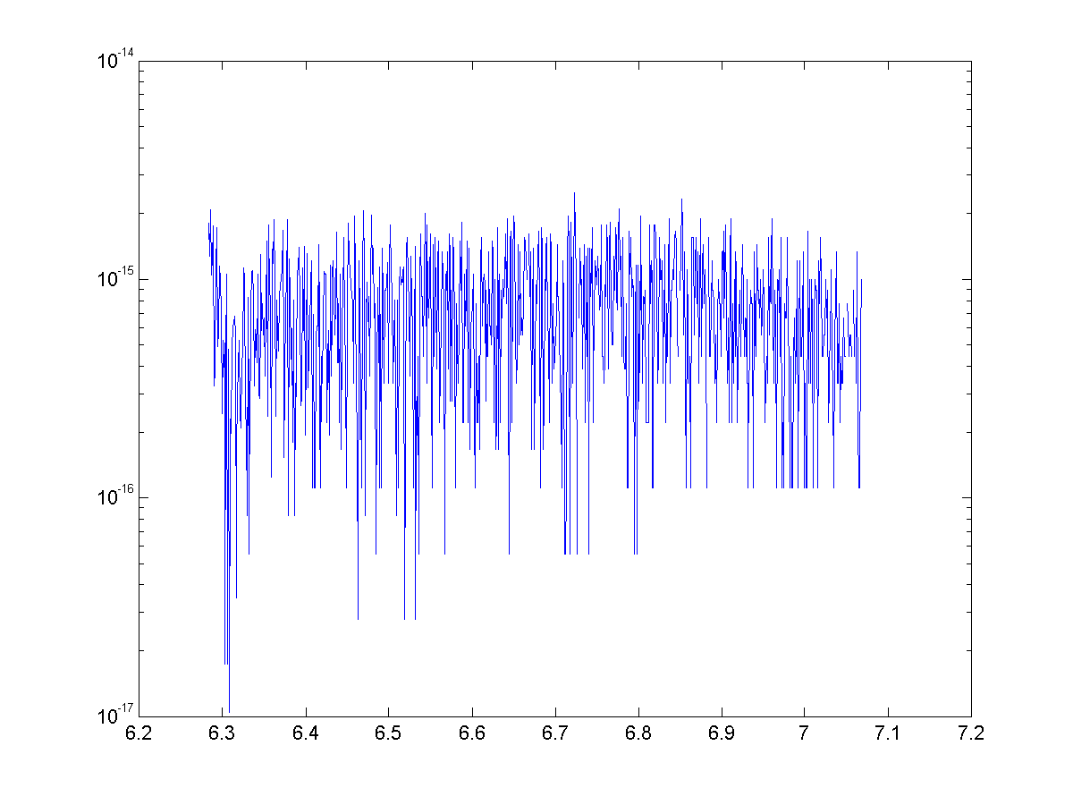
See below for the error for approximations for cosine with 4, 8, 12, and 14 terms. With 14 terms, we are more or less bounded by machine precision (~15 significant figures)
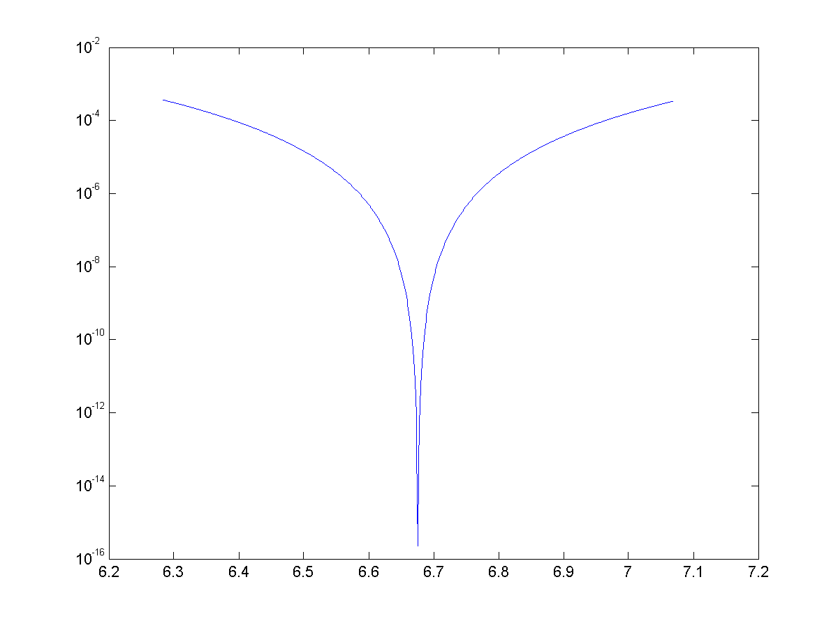
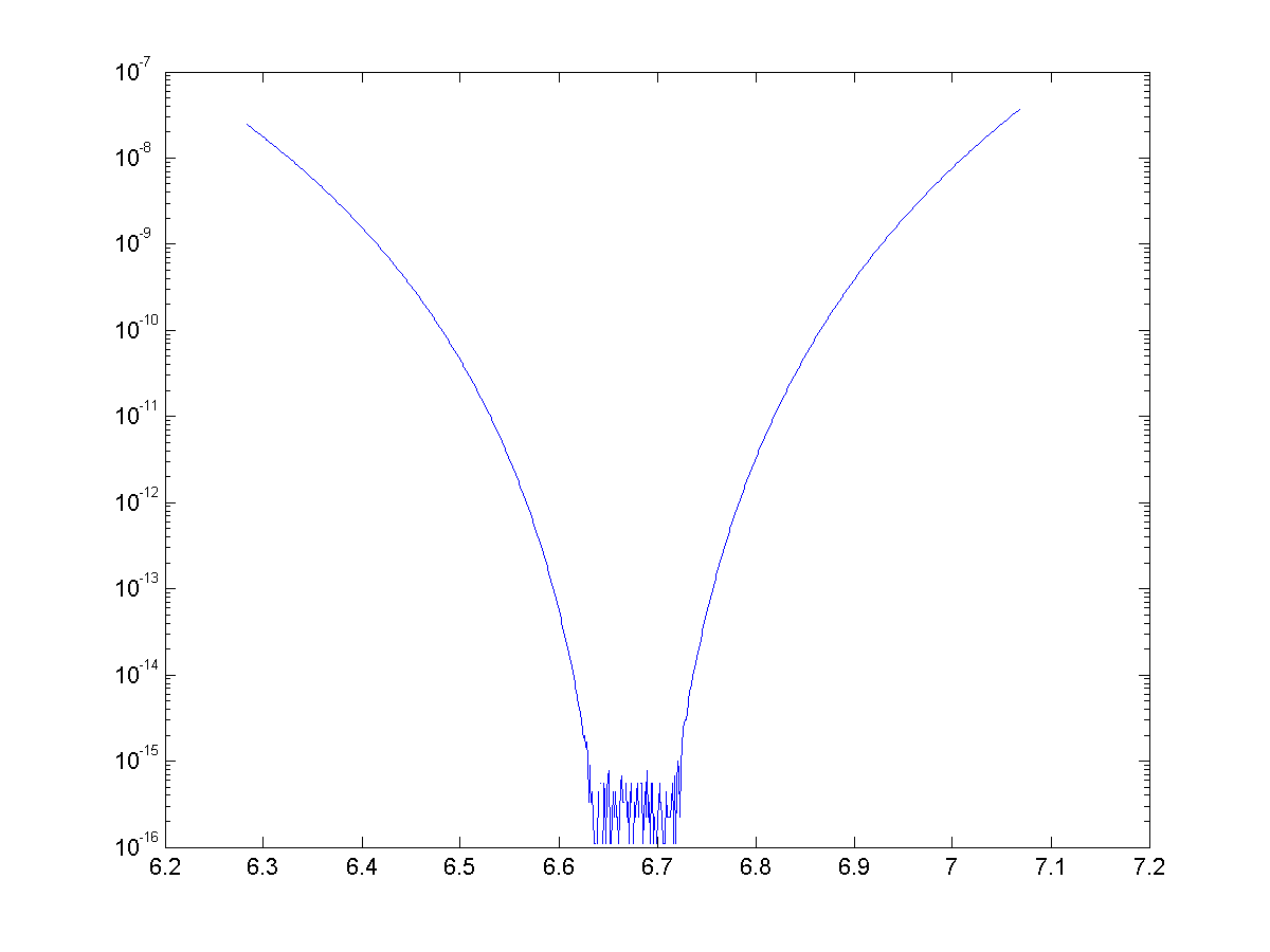
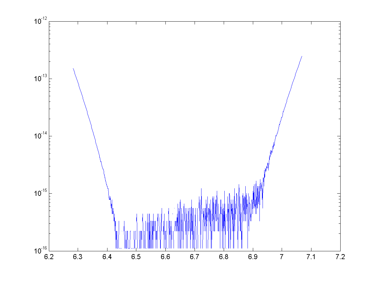
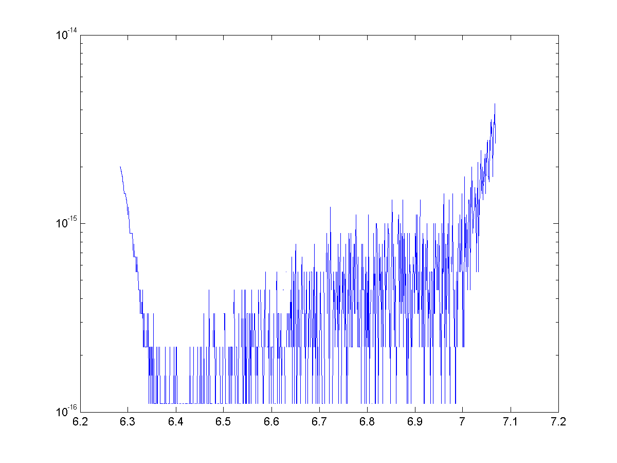
Once again we have generated some exciting looking, but nonetheless useless approximations. We were able to use binomial theorem and some trickery to generate approximations with great accuracy, but once again they are nowhere near as speedy to calculate as the Maclaurin series.
Representing Trigonometric Functions with the Binomial Series
Posted on April 4, 2014
In this post, we will introduce the incredibly useful binomial theorem and series, then use the series and De Moivre's theorem to derive a representation and approximations for trigonometric functions.
Background
The binomial theorem is a way to expand a binomial raised to a power. For a natural number $n \in \mathbb{N}$ the binomial theorem is $$ (a+b)^n={n \choose 0} a^n b^0 + {n \choose 1} a^{n-1}b+{n \choose 2} a^{n-2}b^2…+{n \choose n} a^0 b^{n}.$$
A tidier closed form expression is $$ (a+b)^n=\sum_{k=0}^{n}{ {n \choose k} a^{n-k}b^{k} } .$$ Closely related to the binomial theorem (integer exponents) is the binomial series (for non-integer exponents).
For a real exponent $\alpha \in \mathbb{R}$ the binomial theorem becomes: $$ (a+b)^{\alpha}=\sum_{k=0}^{\infty}{ {\alpha \choose k} a^{\alpha-k}b^{k} } .$$ Without getting too in depth on convergence, it is important that $a<b$. The convergence of this series when $a=b$ depends on $\alpha$. There is more on convergence here.
Even if $\alpha$ isn't an integer, the coefficients ${ \alpha \choose k}$ are calculated similarly. Let’s look at two examples.
For integers: $${ 7 \choose 3}=\frac{7\cdot 6\cdot 5}{3\cdot 2\cdot 1}=35.$$ For non-integers: $${ 7.2 \choose 3}=\frac{7.2\cdot 6.2\cdot 5.2}{3\cdot 2\cdot 1}=38.688.$$ The generalized binomial has some useful applications like approximating roots, deriving multiple angle formulas, and approximating $e$.
Deriving a series
The starting point for deriving these series is De Moivre's Theorem. The theorem is most commonly in used complex analysis, but it is probably best known as a tool for deriving multiple angle formulas. This theorem can be found in any complex analysis text, but we will state it here for clarity.
De Moivre's Theorem: For $n\in \mathbb{Z}$ and $\phi \in \mathbb{R}$
In multiple angle formula derivations, $n$ is generally a constant integer and $\phi$ is a variable. However, there are two significant differences in our approximations. We will leave $\phi$ constant and we will replace $n$ with a variable $\alpha \in \mathbb{R}$ that can vary.
In general, De Moivre's Theorem breaks down when generalized to $\alpha \in \mathbb{R}$. Any standard complex analysis book can provide examples of this. The proof is a little dry so we won’t show it here, but It can be shown that as long as we pick $\phi \in (-\pi,\pi]$, our generalization of De Moivre's Theorem holds.
Let $\phi \in (-\pi,\pi]$ with $\phi \neq 0$ and let $\theta=\alpha\phi$ for $\alpha \in \mathbb{R}$. Now we can take this special case of De Moivre's Theorem and apply the generalized binomial theorem, yielding: \begin{eqnarray*} \cos{\theta}+i\sin{\theta}&=&\cos{\alpha\phi}+i\sin{\alpha\phi}\\ &=&(\cos{\phi}+i\sin{\phi})^\alpha \\ &=&\displaystyle\sum_{k=0}^\infty{i^k{\alpha\choose k}\cos^{\alpha-k}{\phi}\sin^{k}{\phi} } \\ &=&\cos^{\alpha}{\phi}\displaystyle\sum_{k=0}^\infty{i^k{\alpha\choose k}\tan^{k}{\phi} }\\ &=&\cos^{\alpha}{\phi}\displaystyle\sum_{k=0}^\infty{(-1)^k\left[{\alpha\choose 2k}\tan^{2k}{\phi}+ i{\alpha \choose 2k+1}\tan^{2k}{\phi}\right]}. \end{eqnarray*} Now we equate the real and imaginary parts: \begin{eqnarray*} \cos{\theta}&=&\cos^{\alpha}{\phi}\displaystyle\sum_{k=0}^\infty{(-1)^k{\alpha\choose 2k}\tan^{2k}{\phi} } \\ \sin{\theta}&=&\cos^{\alpha}{\phi}\displaystyle\sum_{k=0}^\infty{(-1)^k{\alpha \choose 2k+1}\tan^{2k+1}{\phi} }. \end{eqnarray*} We can also create an alternative form by letting $x=\tan\phi \rightarrow \cos\phi=1/\sqrt{1+x^2}$: \begin{eqnarray*} \cos{\theta}&=&\left(1+x^2\right)^{-\alpha/2}\displaystyle\sum_{k=0}^\infty{(-1)^k{\alpha\choose 2k}x^{2k} } \\ \sin{\theta}&=&\left(1+x^2\right)^{-\alpha/2}\displaystyle\sum_{k=0}^\infty{(-1)^k{\alpha \choose 2k+1}x^{2k+1} }. \end{eqnarray*} While we will not go in depth here, it is important to study the convergence of these series. As a general rule, the series will converge for $\phi$ such that $\cos{\phi}>\sin{\phi}$ (this can be verified with the ratio test). It can also be shown with the alternating series test that if $\cos{\phi}=\sin{\phi}$, then the series will converge for $\theta\geq-\pi/4$. Both series converge for the values of $\theta$ and $\phi$ chosen later in this paper.
Approximations
To implement these series as approximations, they must be truncated. The error associated with this truncation is heavily dependent on both $n$, the number of terms in the truncated series, and the value of $\phi$. The number of terms will be predetermined for consistency and computational efficiency. Realistically, values around $n=8$ are a good starting place because the standard approximation for trigonometric functions in MATLAB utilizes a truncated and slightly modified Maclaurin series with $8$ terms.
For the approximations to be repeatable without re-evaluating $\tan{\phi}$ and $\cos{\phi}$, the value of $\phi$ must be constant. With $\phi$ and $n$ constant, $\alpha$ will be recomputed for each $\theta$. Sensitivity studies on $\phi$ showed that approximations with $\tan{\phi}=.1$ are exceptionally accurate for a small number of terms, so that value will be used for approximations throughout the rest of the paper. Let’s try an example.
Example: Approximate $\cos{\pi/3}$.
Solution:Let $\phi=\tan^{-1}({.1})\approx.0997$. Then we compute $\alpha = \frac{\pi/3}{.0997} = 10.5.$ We will use $n=8$ terms in our approximation. We have \begin{eqnarray*} \cos{\pi/3} &\approx& \cos^{10.5}({.0997}) \displaystyle\sum_{k=0}^7{(-1)^k{10.5 \choose 2k}\tan^{2k}({.0997})} \\ &=&\cos^{10.5}({.0997}) \left[ 1-\frac{10.5(10.5-1)}{2!}.1^2+-... \ +-\frac{10.5(10.5-1)...(10.5-13)}{14!}.1^{14} \right] \\ &=&0.49999999999999944.\\ \end{eqnarray*} These approximations cannot be easily evaluated by hand, but can be carried out with a computer quickly and with exceptional accuracy. The outline and basic code for the cosine approximation are below.
- Specify $\phi$ and $n$
- Compute $\alpha$
- Initialize coefficient and sum variables
- Use an iterative loop to calculate the generalized binomial coefficients and new terms
- Multiply the sum by $\cos^\alpha(\phi)$
An example of this code is (written for MATLAB) is
[approx, error] = function calculate_theta(theta)
tan_phi=.1;
phi=0.099668652491162;
cos_phi=0.995037190209989;
alpha=theta/phi;

coeff=1;
n=8;
sum=0;

for i=1:n
    sum=sum+coeff;
    coeff=-tan_phi^2*coeff*(alpha-2*i+1)*(alpha-2*i+2)/(2*i)/(2*i-1);
end

approx=sum*cos_phi^alpha;
error=approx-cos(theta);
Recall, $\phi$ is predetermined, so $\tan{\phi}$ and $\cos{\phi}$ are constants. In this code, they are represented with tan_phi and cos_phi respectively. Also, theta represents $\theta$, alpha represents $\alpha$, n represents the number of terms in the truncated series, coeff is each term in the series, and sum is utilized in the loop to add up the terms.
Before we get too ahead of ourselves, we need to consider how this stacks up against existing approximations for trigonometric functions. The simplest is the Maclaurin Series, with example source code shown here. While our approximations are a novel new look, they take much longer to compute so they are not a viable replacement for any existing approximations.