Drafting Fantasy Football Teams: A Comparison Greedy Algorithms
Posted on September 7, 2015
Fantasy football is an increasingly popular game for American football fans. Coaches compete within a league, typically of friends or coworkers. The standard roster of starters includes 1 QB, 2 RB, 2 WR, 1 TE, 1 D/ST (defense/special teams), 1 K, and 1 F (flex: can usually be a WR, RB, or TE). Teams also have bench players (backups for when starters are struggling or on a bye week).
If you aren’t familiar with how fantasy football works, read more here. Even if you aren’t a big football fan, this is worth learning for the exciting strategy behind playing. From here on out, I will assume you have a basic working knowledge of the game.
There are a lot of week to week strategies that coaches employ to pick up the best players off the waiver wire or win week to week, but for now we will just focus on the draft.
Simple Greedy Algorithm
The simplest way to draft is to just pick the best available player. We will call this a greedy algorithm. There is no negative connotation implied here; it just describes the algorithm design: pick the best player available based on projected points.As it turns out, this strategy isn’t too bad; better than wonky strategies like picking only Jets and Chargers players or only from teams capable of flight (both are strategies I've drafted against). Success in a draft is obviously not guaranteed. After all, only one person can draft the best team. As many seasoned coaches suspect, the lucky coaches with early picks (1-3 overall) are more likely to draft teams with the highest projections.
If you are the poor guy sitting in the back with the last pick, it seems like there’s nothing you can do. Even if you know who your opponents are picking, there is not a clear and intuitive way to leverage that information if you stick to just picking the best available. If only there was a way to take advantage of the knowledge of who other players are picking…and that’s where the predictive greedy algorithm comes in.
Predictive Greedy Algorithm
Let’s think through a modification of the simple greedy algorithm by considering the following situation. Let’s say (hypothetically) that you have the QB and WR positions open. Also, Peyton Manning is the best player available and he is worth 500 points, the next best player available is Calvin Johnson, projected to get 475 points. The simple greedy algorithm would tell you to pick Peyton because he is worth more points. When the next round comes around, Calvin Johnson is no longer available at WR so you have to “settle” on 375 from Brandon Marshall.But wait, there’s more! Let’s also say 3 spots behind Peyton (in QBs) is Philip Rivers, a less popular choice, but still projected to get 425 points. And better yet, you know how you’re opponents pick so you know there is a high chance he’ll be available next round. So you can let Peyton Manning go to another team and pick up Calvin Johnson even though he doesn’t have the highest points available, then get Phillip Rivers the next round(Peyton will surely be gone). Some simple math later, you drafted two players worth a combined 475+425=900 points (Johnson and Rivers) instead of 500+375=875 (Manning and Marshall), because you were able to predict what your opponents were going to do, and exploited it.
With that example in mind, let's formally define our new greedy algorithm. Each pick you will follow these steps:
- Determine the best available player and simulate that you pick him
- Determine the best available player at every other position
- Simulate other coaches picking for a round until the pick comes back to you
- Once again, determine the best available player at every position
- Calculate the position with the highest decrease in points and pick that player
There are some obvious shortcomings to this highly trivialized situation, namely the lack of information. You will never know exactly who you’re opponents are going to pick, and risking big by drafting lower rated players earlier can be dangerous. However, in our academically predictable environment, this strategy proves to be quite fruitful.
Comparison
We are going to simulate 66 different drafts: 6-16 person leagues (by 2’s) with everyone picking with the simple greedy strategy except for one person, who will pick with the predictive greedy algorithm. The code is largely unexciting bookkeeping so I won’t walk through it, but you can find it on GitHub.
As expected, the predictive greedy algorithm is quite successful, particularly in larger drafts and for players in the middle of the draft order.
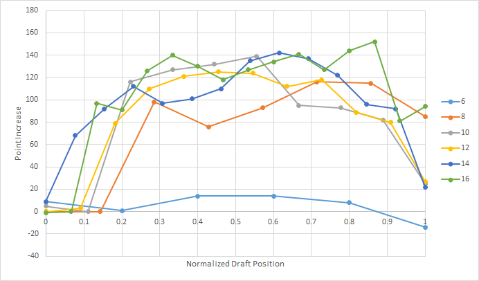
Coaches who picked following this strategy picked the team with the highest projected points 89% of the time.
Other Considerations
This is obviously a drastic oversimplification of the drafting problem, namely because we know our opponents strategy. In reality, coaches’ picks are more sporadic. Some coaches employ strategies like picking 3 RBs in their first 3 rounds, others pick players heavily from their favorite teams.Regardless of how your league tends to pick, a key to success is to get out front of these trends right before they happen (and not too early). We can see the importance of this in the chart below.
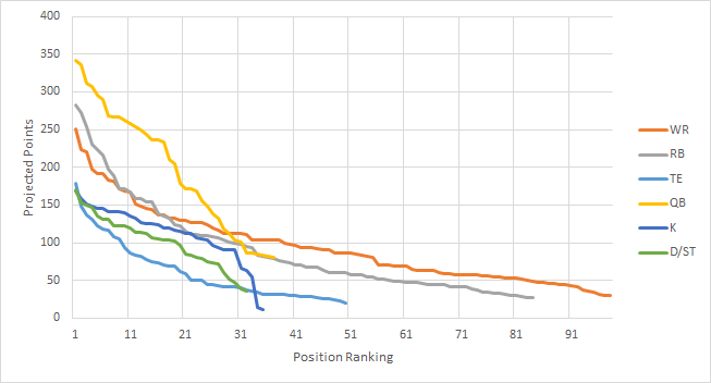
Each position has diminishing point value (the slope flattens out) as you go further out in the rankings, some faster than others. You want to pick anytime when the slope is steep, but on the front end (you don't want to pick after the major drop offs). But not all positions are picked at the same time, and this varies by league. In some leagues, quarterbacks go in the 1st round, in some not till the 5th - some leagues pick defenses in the 5th round and some pick defenses in the 8th round. If you know other coach's tendencies, you can get out in front of these major drop offs and take advantage of them.
This overlooks a few other important details - one of which is the bye week problem. Each player has a bye week some time from Week 4 to Week 11 in the 17 week season. Some coaches hedge against this by spreading out the bye weeks among their team – others try to get all the bye weeks at the same time so their team takes only one bad loss.
Another overlooked assumption comes from picking bench players. Consider a 6-team league. There are far more than six QBs that are fairly evenly matched and good enough to start on a fantasy team. Therefore in this simulation, a coach who waits until the last pick to draft the QB does not suffer too much in points lost. However, in reality, some coaches pick their backup QB quite early; some even draft a backup before they fill in all of their starting positions. This decision-making process is hard to predict in these simulations.
With all the assumptions that have gone into this analysis, it’s unlikely that a coach could replicate this success without a little bit of luck and lot of predictable behavior from their opponents. If you did have this information (looking at you ESPN), there is a lot of potential to take this in exciting new directions.
Implicit finite difference formulation on an unstructured mesh
Posted on March 17, 2014
Introduction
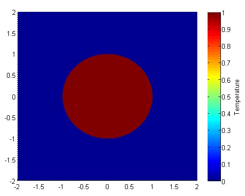
Objective: Obtain a numerical solution for the 2D Heat Equation using an implicit finite difference formulation on an unstructured mesh in MATLAB. The temperature distribution over time for an example problem described below will look something like this:
Helpful background: basic understanding of PDEs (partial differential equations), basic MATLAB coding (for loops, arrays and structure arrays), and solution methods for matrix equations.
Modeling the physics
First let’s introduce the heat equation. The heat equation in two dimensions is $$u_t=\alpha(u_{xx}+u_{yy})$$ where $u(x,y,t)$ is a function describing temperature and $\alpha$ is thermal diffusivity.
Numerically discretizing the equations We are going to solve the heat equation numerically with finite differences on an unstructured mesh. This is a fairly non-standard approach; when numerical analysts encounter difficult geometries they typically move on from cartesian finite difference for coordinate transformations, or other methods like finite volumes or finite elements on unstructured meshes.
We will keep as close as possible to the true nature of finite difference without using coordinate transformations. Our previous post did this as well, but what makes this method more desirable is the flexibility that comes from unstructured meshing. With an unstructured mesh, it is easier to mesh around complex geometries and add local refinement.
Approximating derivatives To create discretized equations we will need approximations for the second derivatives $u_{xx}$ and $u_{yy}$. We will go back to a Taylor series expansion, but this time extend it in in two dimensions. Consider a function $u$ at points $u_0=u(x_0,y_0)$ and $u_1=u(x_1,y_1)$ with $x_1=x_0+\Delta x$ and $y_1=y_0+\Delta y$. Then the two dimensional Taylor series expansion is $$ u_1 \approx u_0 + u_x\Delta x +u_y\Delta y +u_{xx}\Delta x^2 +u_{yy}\Delta y^2 +u_{xy}\Delta x \Delta y $$ We will treat $\Delta x$, $\Delta y$, $\Delta x^2$, $\Delta y^2$, $\Delta x\Delta y$, as coefficients and let the derivatives be the unknowns. Then we have a linear equation with five unknowns, $u_x$, $u_y$, $u_{xx}$, $u_{yy}$, and $u_{xy}$. That means to solve for all first and second derivatives requires five linearly independent equations, which we can get if we have $n \geq 5$ neighboring points that aren't collinear in the same direction.
Set it up as $A\textbf{x}=\textbf{b}$ where \[ \textbf{b} = \left[ \begin{array}{c} u_1-u_0 \\ u_2-u_0 \\ … \\ u_n-u_0 \end{array} \right] \] \[ \textbf{x} = \left[ \begin{array}{c} u_x \\ u_y \\ u_{xx} \\ u_{yy} \\ u_{xy} \\ \end{array} \right] \]
and $A$ is the coefficient matrix.
As one might guess, this results in approximations with second order accuracy for the first derivatives but only first order accuracy for the second derivatives, which is not acceptable accuracy. There are different ways to address this but the simplest is to add the third derivative terms to our equations. There are four third derivatives $u_{xxx}$, $u_{yyy}$, $u_{xxy}$, and $u_{xyy}$. This means we will need to use information from nine neighboring points to attain second order accuracy.
Now you may be wondering, how will we pick the nine neighboring points that best solve the physical problem? To best capture the physics we want equal weight from the surrounding points. However, unstructured meshes have a varying number of neighboring points, and often times have less than nine. To address this problem we will get greedy - we will not take just all neighboring points, but all the neighbors of neighboring points. This will leave us with much more than nine equations (generally 20-30) for only nine unknowns.
To best solve the overdetermined system we will use the least squares method. For an overdetermined system $A\textbf{x}=\textbf{b}$ the least squares solution is $$ \textbf{x}=\left[ (A^TA)^{-1}A^T \right] \textbf{b}$$ Let $\textbf{d}$ be the sum of the fourth and fifth rows of $(A^TA)^{-1}A^T$. Then we can write $$ (u_{xx}+u_{yy})_{x_0,y_0} = \textbf{d}\textbf{b}.$$ Since the mesh does not move we can use the same coefficients to calculate derivatives at every time step. Therefore these least squares calculations and assembly $\textbf{d}$ vectors (one for each node) of only need to be carried out once.
As we will show later in the code it is not good if the matrix has linearly dependent rows. To avoid this one could add an error check that eliminates $\Delta x$ and $\Delta y$ pairs that have close to the same angle. The closer points are to being linearly independent, the worse the condition of the matrix $A$. That said, if the angles differ by $180^{\circ}$ then rows are still linearly independent due to the nature of the coefficients.
Now that we have a way to calculate the derivatives, we can implement a formulation. We have shown the explicit FTCS formulation in two previous posts, so in this post we will just focus on an implicit method. We will use the Crank-Nicolson method (for more, check this paper on finite differences with the heat equation).
Implicit formulation (Crank-Nicolson)
The approximation becomes \begin{eqnarray} u_t^n &=& \alpha\cdot(u_{xx}+u_{yy}) \\ \frac{u^{n+1}-u^n}{dt} &=& \frac{\alpha}{2} \left[ (u_{xx}+u_{yy})^{n+1} + (u_{xx}+u_{yy})^n \right] \\ u^{n+1} - \frac{\alpha\cdot dt}{2}(u_{xx}+u_{yy})^{n+1} &=& u^n + \frac{\alpha\cdot dt}{2}(u_{xx}+u_{yy})^n \\ u^{n+1} - \frac{\alpha\cdot dt}{2} \textbf{d}\textbf{b}^{n+1} &=& u^n + \frac{\alpha\cdot dt}{2} \textbf{d}\textbf{b}^n \end{eqnarray} The left hand side of the equation is called the implicit side and contains the unknowns $u^{n+1}$ and $\textbf{b}^{n+1}$. The right hand side is all known values ($u^n$ and $\textbf{b}^n$ are from the previous time step) and is called the explicit side.
If we create an equation like this for each of the $n$ point in our domain then we have a system of $n$ equations with $n$ unknowns in the form $A\textbf{x}=\textbf{b}$ where $\textbf{x}$ is all of the $u^{n+1}$ values, $\textbf{b}$ is the explicit side, and $A$ is the coefficients from the left hand side.
Example problem
For example we will use the same physical problem as in part 2 (the only difference is the length scale). A $1x1$ flat plate has a thermal diffusivity of $\alpha=.001$. The temperature is fixed at $u=1$ on an inner circular boundary and is fixed at 0 on four outer boundaries. Elsewhere, the initial temperature is $u=0$. Find the temperature distribution over time.
Meshing
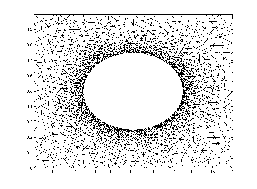
Much of the best meshing software is propietary and expensive, but there are some good free programs like Gmsh. We will implement code to read in and use a *.msh file.
We will test out the mesh below. It has $1,992$ nodes.
The code
Now let’s lay out the code. We are going to break it up into three steps: initialize relevant physical parameters, import the mesh, set the boundary conditions, assemble the coefficient matrix, and set up the time loop.
Step 1: Initialize physical parameters
%Physical Quantities
nts=100; ntsabout=100;
dt=.03; alpha=.001; c=alpha*dt/2;
Step 2: Import the Mesh
[xyz,mesh,nn,tri,bnd,map]=importmesh2('circle_fine.msh');
The function will return
- xyz: the nodes in a (nn,2) where nn is the number of points in the mesh.
- mesh: A structure array containing the fields nbr (neighboring points), dx and dy (the distances to respective points), coeff the coefficients of the derivative approximation, and bnd, the boundary type of the point.
- tri: the “connectivity of the mesh (for visualizations).
- nn: The number of nodes in the mesh
- bnd: a list of the nodes in the boundary. Only necessary for an implicit formulation.
- map: The points in the mesh not on a boundary.
I will not include the importmesh2 code in this post but you can access the text here.
Step 3: Apply Initial and Boundary Conditions
%Initialize arrays
T = zeros(nn,1); A=zeros(nn); b=zeros(nn,1);

%Initial conditions
for n=bnd
    if mesh(n).bnd==5
        T(n)=1;
    end
end
Step 4: Assemble coefficient matrix and boundary contribution to the rhs vector
for i=bnd
    A(i,i)=1;
end

for i=map
    A(i,i)=1+c*mesh(i).coeff(end);
    for j = 1:length(mesh(i).nbr)
        A(i,mesh(i).nbr(j))= -c*mesh(i).coeff(j);
    end
end

b(bnd)=T(bnd);
Step 5: Time Loop
for t=1:nts
    %update rhs
    for n=map
        dd=mesh(n).coeff*[T(mesh(n).nbr); -T(n)];
        b(n)=c*dd+T(n);
    end

    %solve matrix equation
    %T=Ai*b;             %use inverse of A, requires Ai=inv(A)
    %T=A\b;              %MATLAB built in mldivide
    %T=L\T; %T=U\T;      %LU decomposition, requires [L,U]=lu(A);
    [T,flag]=gmres(A,b); %GMRES method

    %update visualization
    if mod(t,ntsabout)==0
        trisurf(tri,xyz(:,1),xyz(:,2),T,'FaceColor','interp','EdgeColor', 'none')
        axis([0,1,0,1]); view(0,90); colorbar; grid off;
        outframe(t) = getframe;
    end
end %time loop
Results
We already showed a visualization at the top of the post so let's look at run-time comparison of explicit and a few different matrix solver methods with implicit. The methods are explicit (FTCS), MATLAB’s mldivide (\), $LU$ decomposition with back-substitution, inverting $A$, and the GMRES method. We used the mesh shown above and a refined mesh with four times as many nodes. We calculated two time lengths, $3~\mathrm{s}$ and $30~\mathrm{s}$. Computation times are given in seconds.
| Method | $t=3~\mathrm{s}$ (coarse) | $t=30~\mathrm{s}$ (coarse) | $t=3~\mathrm{s}$ (fine) | $t=30~\mathrm{s}$ (fine) |
|---|---|---|---|---|
| Explicit | 11.94 | 121.30 | N/a | N/a |
| A\b | 42.28 | 411.5 | N/a | N/a |
| LU | 2.50 | 25.04 | 35.35 | 184.5 |
| Inversion | 1.72 | 17.08 | 67.42 | 146.8 |
| GMRES | 2.76 | 24.18 | 29.71 | 225.3 |
Since the coefficient matrix doesn’t change with every time step, the speed during the time loop is greatly increased by inverting $A$ or determining its $LU$ decomposition beforehand. The GMRES method on the other hand, is fast because it is designed to handle sparse matrices like $A$.
We are only able to get away with inverting $A$ because our mesh is very small. Matrix inversion is a computationally expensive operation that does not scale well (see here). For example, if one quadruples the mesh points as we have, the run time for inverting $A$ theoretically increases by a factor of 64. Furthermore MATLAB documentation recommends against using the inv command whenever possible. The $LU$ decomposition is generally considered to be better practice than inversion, but it also scales poorly for large matrices unless an algorithm that takes advantage of the sparse nature of $A$ is employed.
In a reasonably large computation, GMRES would generally be the best method unless another method can be employed that efficiently inverts sparse matrices (such methods exist for specialized problems).
Structured, transformation-free finite differences on complex geometries
Posted on January 22, 2014
Introduction
Objective: Obtain a numerical solution for the 2D Heat Equation on mesh with circular boundaries in MATLAB using an explicit finite difference formulation with Richardson extrapolation (and without coordinate transformation).
Helpful background: A basic understanding of PDEs (partial differential equations), MATLAB coding (for loops, arrays, functions, maps, trisurf, and bitget), basic derivative approximations with finite differences and Richardson extrapolation.
Modeling the problem
First let’s introduce the heat equation. The heat equation in two dimensions is $$u_t=\alpha(u_{xx}+u_{yy})$$ where $u(x,y,t)$ is a function describing temperature and $\alpha$ is thermal diffusivity.
Numerically discretizing the equations We are going to solve the heat equation numerically with an explicit formulation. We talk about this a little in our previous post on the heat equation. There are many methods that solve this, but the simplest is an explicit finite difference formulation. The major difference here is how we handle the more difficult geometry of a circular disk. If none of the points neighbor the boundary, we will use the central difference approximation for our second derivatives. The approximations for $u_{xx}$ and $u_{yy}$ are \begin{eqnarray} u_{xx}(i,j)=\displaystyle\frac{u(i+1,j)-2\cdot u(i,j)+u(i-1,j)}{(\Delta x)^2} \\ u_{yy}(i,j)=\displaystyle\frac{u(i,j+1)-2\cdot u(i,j)+u(i,j-1)}{(\Delta y)^2}. \end{eqnarray}
Calculating the second derivatives for points near boundaries with curvature will be covered in the next two sections.
We will then update the temperature using a first derivative forwards in time. $$ u_t^n=\frac{u^{n+1}-u^n}{\Delta t}.$$ The final formulation is then \begin{eqnarray} u^{n+1}(i,j) &=& u^n(i,j)+\alpha\cdot \Delta t\cdot \left(u_{xx}^n(i,j)+u_{yy}^n(i,j)\right) \end{eqnarray}
Geometries with Curvature When geometries become more complex than a 1D problem on a line or a 2D cartesian grid, many numerical analysts move on to one of three methods: finite volume methods, finite element methods, or finite difference methods with coordinate transformations. These formulations are much more difficult to implement, but can essentially handle any geometry (with varying difficulty).
Instead of using one of these methods we will stick with finite differences and take advantage of a tool call Richardson extrapolation to keep the second order accuracy that led to a nice solution in Part 1.
Let’s set up a specific example. A $4x4$ flat plate has a thermal diffusivity of $\alpha=.01$. The temperature is fixed at $u=1$ in an inner circle with radius $1$. Elsewhere, the initial temperature is $u=0$ and the outer boundaries are fixed at $u=0$ for all time. Find the temperature distribution over time.
(Note: I left off any units and have some simplified numbers for temperature and plate dimensions. Feel free to change them as you please, but make sure your formulation is still stable.)
The initial condition would look something like this:
Richardson Extrapolation Before we get started, it may help to glance at some of the basics of Richardson Extrapolation at Wikipedia.
The biggest challenge in our problem is that it requires a second derivative, which proves to be a little harder to compute with second order spatial accuracy. First and foremost, we can’t do it with just the two neighboring points (like we would be able to with evenly spaced points); we will need to use one more. Consider the points below. Assume that at each point $1,2,3,4$ we know the value of a function $f$ are $f_1,f_2,f_3,f_4$.
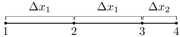
We will use information at the points $1,2,3,$ and $4$ to approximate the second derivative at point $3$, $f_3^{\prime\prime}$ . Why point $3$? In our particular problem, the second derivatives at points $1$ and $2$ can be approximated with a standard central difference and point $4$ will be a boundary, so the second derivative will not need to be calculated there.
Our first step will be to calculate the first derivatives at points $2,3,$ and $4$. These are fairly straightforward; we will use a central difference at point $2$ and Richardson extrapolation and points 3 and 4. They should look something like this \begin{eqnarray} f_2^{\prime} &=& \displaystyle\frac{f_3-f_1}{2\cdot \Delta x_1} \\ f_3^{\prime} &=& \displaystyle\frac{k_1\cdot (f_4-f_3)}{(k_1+1)\cdot \Delta x_2}+\frac{(f_3-f_2)}{(k_1+1)\cdot\Delta x_1} \\ f_4^{\prime} &=& \displaystyle\frac{k_2\cdot (f_4-f_3)}{(k_2-1)\cdot\Delta x_2}-\frac{f_4-f_2}{(k_2-1)\cdot (\Delta x_1+\Delta x_2) } \end{eqnarray} Where $k_1= \frac{ \Delta x_1}{ \Delta x_2}$ and $k_2=\frac{ \Delta x_1+ \Delta x_2}{ \Delta x_2}$ . Now we will use these to approximate the second derivative at $x_3$ with Richardson extrapolation. This is very similar to the formula except we will use a different value of $k$, namely $k_3=\frac{4\cdot k_1-1}{2\cdot k_1-2}$.
After wading through the algebra, your expression will simplify to $$f_3^{\prime\prime} = \frac{\Delta x_2^3\cdot (f_1-2 f_2+f_3)+\Delta x_1^3\cdot (6 f_4-6 f_3)+\Delta x_1^2\cdot \Delta x_2\cdot (-f_1+8 f_2-7 f_3)}{\Delta x_1^2\cdot \Delta x_2\cdot (\Delta x_1+\Delta x_2)\cdot (2 \Delta x_1+\Delta x_2)} $$
This is a pretty costly formula compared to the central difference method. Fortunately, we will not have to use this equation very often; only when the points are neighboring the boundary. Meanwhile, this allows us to use the cheap and effective central difference method at all other points. Therefore the overall computation should be fairly inexpensive.
We will also need to generate a mesh. Below is an example of the mesh. The elements have been triangulated for simple viewing in MATLAB, but there is no triangulation and no element formulation in the solution.
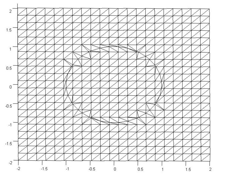
The original mesh here was a $22x22$ grid, but there were an additional 40 points added on the boundary to maintain the curvature of the circle. The important part is finding the $\Delta x_2$ and $\Delta y_2$ values for each of the points immediately neighboring a boundary and creating an additional point on the mesh.
When we loop through the mesh points we will ignore all points where the temperature is specified, use Richardson Extrapolation on the points adjacent to the 40 added points, and uses central differences elsewhere.
A Quick Look at Stability In the previous part we discussed stability, namely that in order for the old formulation to hold we needed to satisfy $$ \Delta t < \frac{\Delta x_1^2}{4\alpha}.$$ We will not perform a proper stability analysis, but our empirical results show that $$ \Delta t < \frac{\Delta x_1\cdot min(\Delta x_2)}{4\alpha}$$ is generally sufficient. Once you have your code written it is easy to empirically test different values of $\Delta t$.
The code
We are going to break it up into five steps: Create the Richardson extrapolation function, initialize relevant physical values, generate the mesh, set the boundary conditions, and set up the time loop. The time loop will consist of calculating the derivatives at each point, updating the temperature for each point, and then updating the visualization.
Step 1 Richardson Extrapolation
function [ddf3a] = richardson(dx1,dx2,f1,f2,f3,f4)
ddf3a = (dx2^3*(f1-2*f2+f3) + ...
         dx1^3*(6*f4-6*f3) + ...
         dx1^2*dx2*(-f1+8*f2-7*f3))...
       /(dx1^2*dx2*(dx1+dx2)*(2*dx1+dx2));
end
Step 2 Initialize variables
%Initialize Physical Values
dt=.01;                     %time step
nts=500;                    %number of time steps
alpha=.01;                  %thermal diffusivity
bounds=[-2 2 -2 2];         %corners of outer domain

%Mesh Variables
nx=50; ny=50;               %number of points in the x and y directions
%distance in between points
dx1=(bounds(2)-bounds(1))/(nx-1);
dy1=(bounds(4)-bounds(3))/(ny-1);
Step 3 Generate the Mesh
[xyz,skip,dx2,dy2,tri]=genmesh(bounds,nx,ny);

%The derivatives and temperature will be stored in a 1D arrays
nodes=length(skip);
uxx=zeros(nodes,1); uyy=zeros(nodes,1); T=zeros(nodes,1);
The function will return
- xyz: the nodes in a (np,2) where np is the number of points in the mesh.
- skip: an array that shows whether a point is on a boundary or neighboring one.
- dx2 and dy2: maps relating the distance from a point to the boundary if it neighbors the boundary.
- tri the “connectivity" of the mesh.
An alternative to creating your own tri connectivity would be using the MATLAB built in function tri=delaunay(x,y) but it will not look as good as if you make it yourself.
I will not include any of the code in this post (my version is 160 lines long and it is mostly boring) but you can access the text here.
Step 4 Apply Initial and Boundary Conditions
for p=1:length(skip)
    if skip(p) < 0
        u(p)=1.0;
    else
        u(p)=0.0;
    end
end
Step 5 Time Loop The time loops has three components, first calculate the second derivatives, then update temperature, then update the visualization.
One note before we get into the code. We are using the MATLAB function “bitget” which determines based of the values of skip(p) (see Step 3) whether it is close to the boundary. This is by all means not necessarily the best way to determine whether a point neighbors a boundary, but it works and is not too costly.
for t=1:nts
    for i=2:ny-1
        for j=2:nx-1
            p=nx*(i-1)+j;
            if skip(p) < 0
                continue
            end
            if     bitget(skip(p),1)==1
                uxx(p)=richardson(dx1,abs(dx2(p)),u(p-2),u(p-1),u(p),T_b);
            elseif bitget(skip(p),3)==1
                uxx(p)=richardson(dx1,abs(dx2(p)),u(p+2),u(p+1),u(p),T_b);
            else
                uxx(p)=(u(p-1)-2*u(p)+u(p+1))/dx1^2;
            end

            if     bitget(skip(p),2)==1
                uyy(p)=richardson(dy1,abs(dy2(p)),u(p-2*nx),u(p-nx),u(p),T_b);
            elseif bitget(skip(p),4)==1
                uyy(p)=richardson(dy1,abs(dy2(p)),u(p+2*nx),u(p+nx),u(p),T_b);
            else
                uyy(p)=(u(p-nx)-2*u(p)+u(p+nx))/dy1^2;
            end
        end
    end

    for i=2:nx-1
        for j=2:ny-1
            p=nx*(i-1)+j;
            if skip(p)<0
                continue
            end
            u(p)=u(p)+alpha*dt*(uxx(p)+uyy(p));
        end
    end
    trisurf(tri,xyz(:,1),xyz(:,2),u,'FaceColor','interp');
    frame = getframe(1);
end
Results
Below are two animations of the temperature distribution over time.
Some notes about the code
If you are a novice programmer, you may not have heard of maps. Maps are "objects with keys that index to values" (see here and here). They are similar to an array, except that keys must be unique, keys don't need to be integers, and key values typically aren't ordered. A map is by no means necessary here, but it is an efficient way to store and quickly retrieve the $\Delta x_2$ and $\Delta y_2$ values.
The most confusing part of the code above is implementation of the skip array with bitget. Basically, skip is an array with an integer for every node.
- If a node p is on or inside the circle, skip(p)=-1.
- If it is outside the circle and not adjacent to it, skip(p)=0.
- If it is adjacent to the circle (left, below, right, above) then we add 1,2,4,8 respectively to skip(p). For example, if a point is below and to the right of points on the circle, then skip(p)=6.
We can then reverse engineer skip(p) with bitget. This is not necessarily the best or only way, but it is a relatively simple implementation.
You can save some space in memory by letting uxx and uyy be single values instead of arrays. This however, would either require two arrays for temperature (an old and a new) or some algorithm to keep from overwriting old values of temperature before all derivatives are calculated. Since we are dealing with a relatively coarse 2D mesh, this is not a significant issue.
Finite Difference Solution of the Heat Equation on a Structured Mesh
Posted on November 19, 2013
Introduction
In this post we will numerically solve the heat equation with an explicit finite difference formulation.
Objective: Obtain a numerical solution for the 2D Heat Equation in MATLAB using an explicit finite difference formulation.
Helpful background: basic understanding of PDEs (partial differential equations), basic MATLAB coding (for loops and arrays), and basic derivative approximations with finite differences.
Modeling the problem
First let’s introduce the heat equation. The heat equation in two dimensions is $$u_t=\alpha(u_{xx}+u_{yy})$$ where $u(x,y,t)$ is a function describing temperature and $\alpha$ is thermal diffusivity.
Numerically discretizing the equations We are going to solve the heat equation numerically. There are many methods that solve this, but the simplest is an explicit finite difference formulation. Explicit means the solution at a certain time step depends only on previous step, as opposed to implicit (see here) where the solution depends on next time step. Finite differences are a simple way to use neighboring grid points to approximate derivatives.
We will use the central difference approximation for our second derivatives. The approximations for $u_{xx}$ and $u_{yy}$ are \begin{eqnarray} u_{xx}(i,j)&=&\displaystyle\frac{u(i+1,j)-2\cdot u(i,j)+u(i-1,j)}{(\Delta x)^2} \\ u_{yy}(i,j)&=&\displaystyle\frac{u(i,j+1)-2\cdot u(i,j)+u(i,j-1)}{(\Delta y)^2}. \end{eqnarray} These are all at time $n$ (they are not exponents). We will use the forward difference approximation for $u_t$. We have
$$ u_t^n=\frac{u^{n+1}-u^n}{\Delta t}.$$
This is for every point $(i,j)$. Now we can take these 3 expressions, combine them, and solve for $u^{n+1}$.
\begin{eqnarray} u_t^n(i,j) &=& \alpha(u_{xx}^n(i,j)+u_{yy}^n(i,j)) \\ \frac{u^{n+1}(i,j)-u^n(i,j)}{\Delta t} &=& \alpha\left[\frac{u(i+1,j)-2\cdot u(i,j)+u(i-1,j)}{(\Delta x)^2}+ \frac{u(i,j+1)-2\cdot u(i,j)+u(i,j-1)}{(\Delta y)^2}\right] \\ u^{n+1}(i,j) &=& u^n(i,j)+\alpha\cdot dt\left[ \frac{u(i+1,j)-2\cdot u(i,j)+u(i-1,j)}{(\Delta x)^2}+\frac{(u(i,j+1)-2\cdot u(i,j)+u(i,j-1)}{(\Delta y)^2}\right] \end{eqnarray}
A quick look at stability The formulation we used (forward in time, centered in space) is only conditionally stable. We can show (but won’t here) with Von Neumann Stability Analysis, that we need the discretized time step $\Delta t$ to satisfy $$ \Delta t< \frac{\Delta x^2}{4\alpha}.$$Once you have your code written it is easy to empirically test this.
The code
Let’s set up a specific example. A $1x1$ flat plate has a thermal diffusivity of $\alpha=.01$. The temperature is fixed at $u=1$ on the top and right edges and $u=0$ on the bottom and left edges. Elsewhere, the initial temperature is $u=0$. Find the temperature distribution over time.
(Note: I left off any units and have some simplified numbers for temperature and plate dimensions. Feel free to change them as you please, but make sure your formulation is still stable.)
Now let’s lay out the code. We are going to break it up into three steps: Initialize relevant physical values, set the boundary conditions, and set up the time loop. The time loop will consist of calculating the derivatives at each point, updating the temperature for each point, and then updating the visualization.
Step 1: Initialize variables We will start by initializing relevant physics variables for the time step size, number of time steps, thermal diffusivity, reference plate length, number of points in the x and y direction, and the spatial discretization $\Delta x$ and $\Delta y$.
You can also preallocate the matrices for $u$, $u_{xx}$, and $u_{yy}$.
%Initialize Variables
dt=.005;                   %time step
nts=500;                   %number of time steps
alpha=.01;                 %thermal diffusivity
l=1;                       %reference length plate
nx=50; ny=50;              %number of points in the x and y directions
dx=l/(nx-1); dy=l/(ny-1);  %discretized distance in between points

%Temperature and the derivatives will be stored in a two dimensional array
u = zeros(nx,ny); uxx = zeros(nx,ny); uyy = zeros(nx,ny);
Step 2: Apply Initial and Boundary Conditions
%Initial/Boundary Conditions
for i=1:ny
   u(1,i)=1;
end

for i=1:nx-1
   u(i,ny)=1;
end
Step 3: Time Loop Here is the meat of the code. The time loops has three components, first calculate the second derivatives, then update temperature, then update the visualization.
for t=1:nts
   %Calc the Spatial 2nd Derivative, Centered in Space
   for i=2:nx-1
      for j=2:ny-1
         uxx(i,j)=(u(i+1,j)-2*u(i,j)+u(i-1,j))/(dx)^2;
         uyy(i,j)=(u(i,j+1)-2*u(i,j)+u(i,j-1))/(dy)^2;
      end
   end

   %Update Temperature, Forwards in Time
   for i=2:nx-1
      for j=2:ny-1
         u(i,j)=u(i,j)+alpha*(uxx(i,j)+uyy(i,j))*dt;
      end
   end

   %Visualization
   contourf(u)
   axis equal
   M(t) = getframe;
end %time loop
Results
Below are 2 GIFs (one is a contour plot, the other is a surface plot) of the temperature distribution over time.