Probabilistic Availment
Posted on December 18, 2019
Introduction
This post will tackle two probability questions inspired by a recent Civil Procedure practice test I took. Consider a company that randomly buys $300$ loans from houses all over the United States. What is the probability that at least one of the loans is for a house in Florida? What is the probability that there is a loan for at least one house in each of the fifty states?
The legal purpose for this analysis is determining purposeful availment, a murky part of personal jurisdiction summarized (over)simply enough as "if you meant to business in a certain state, you can be sued there." If a business only had $50$ loans, then they could make a much better case that they don't intend to be subject to a particular state. But for a large number like $300$, intuition tells you that the likelihood is much higher.

Is Florida Targeted?
For the sake of simplicity, assume each state is targeted with equal probability. You could recast the problem as $300$ state quarters if it helps get over the hump of population difference between states like Wyoming and California.
If there was just one state, the probability that it isn't Florida is $\frac{49}{50}=.98$. Similarly, if $300$ states are selected, the probability none are Florida is just $.98^{300}$. So the probability that at least one is Florida is the complement:
$$ 1-.98^{300} = 99.8\%.$$With this many loans there is high certainty that Florida is at least one of them. Side note: $99\%$ may not be high enough, read the top of page 20 of Justice Kagan's dissent in the recent SCOTUS gerrymandering case. Apparently $99\%$ wasn't good enough for the majority.
So how many are loans are sufficient for $50\%$, $95\%$, or $99.7\%$ certainty? This is a simple exercise in logarithms. Let there be $n$ loans and a certainty $p$. Then
\begin{eqnarray*} 1-.98^n &=& p \\ .98^n &=& 1-p \\ \log(.98^n) &=& \log(1-p) \\ n\log(.98) &=& \log(1-p) \\ n &=& \frac{\log(1-p)}{\log(.98)} \\ \end{eqnarray*} So for $p=50\%$ you need $n=35$ houses, $p=95\%$ you need $n=149$ houses, and for $p=99.7\%$ you need $n=288$ houses.Is Every State Targeted?
This is a considerably harder problem. We must consider significantly more cases than just Florida's absence. First, we can tackle it with a simulation for some perspective. The following code does the trick.
import random

num_simulations = 10000
num_states = 50
num_loans = 300
count = 0

for _ in xrange(num_simulations):
    coll = set([])
    for _ in xrange(num_loans):
        coll.add(random.randrange(num_states))

    if len(coll) == 50:
        count += 1

print count/float(num_simulations)
This is helpful, but not satisfying. Can we solve this analytically?
My first intuition was an extension of the previous section, just take the probability of one state and multiply it out 50 times, $\left(1-.98^{300}\right)^{50}$. Unfortunately, there is an oversight here. The discrepancy is hard to spot with $50$ states, but becomes more and more apparent as the problem is recasted with fewer states.
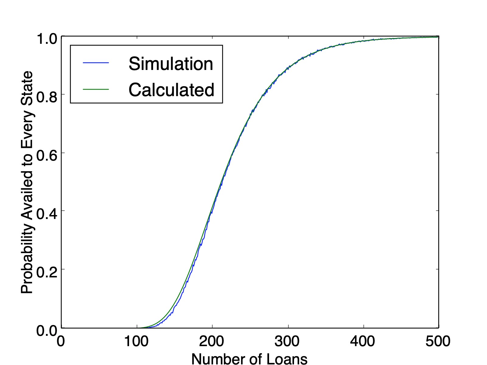
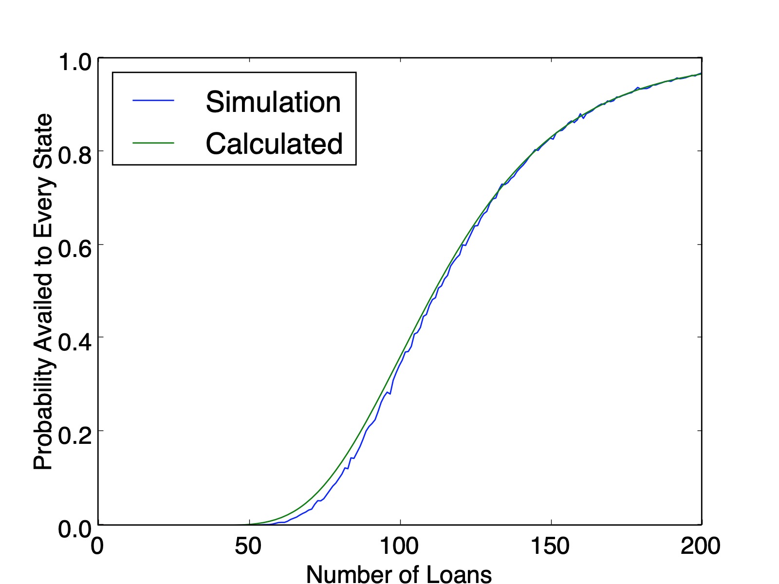
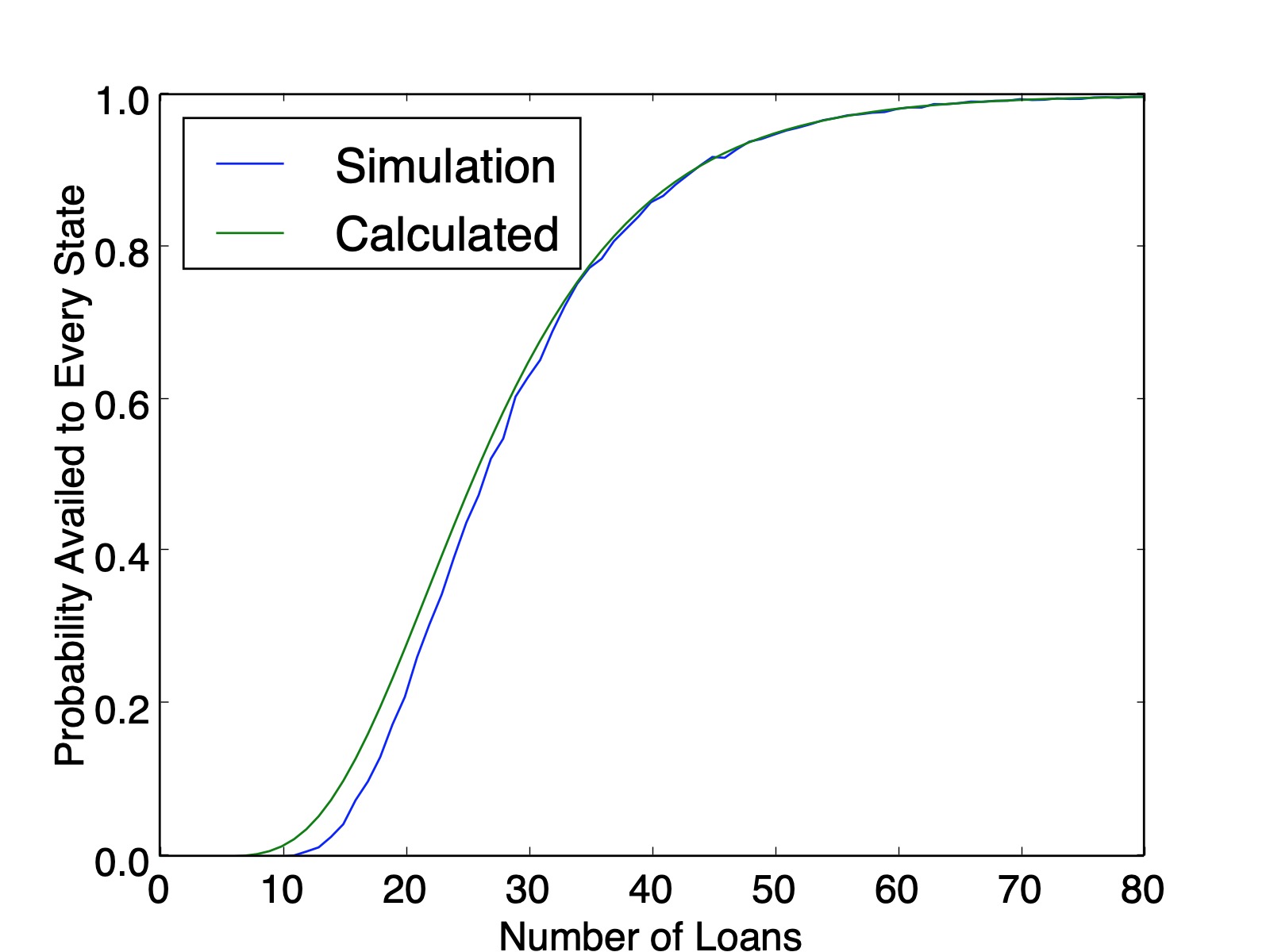
The issue here is that after you determine that Florida is present in the list and you try to move on to next state, that subsequent probability is constrained by how many times Florida came up in the first pass through the list. This dependence cascades down with combinatorial complexity.
Counting a Simpler Case
For illustrative purposes, let's walk through a simpler case, $3$ states and $5$ loans. This will "prove" the accuracy of the simulation and lay out the means for (and complexity of) an algorithm to tackle larger numbers.
There are $3^5=243$ possible ways for the loans to be divided up. We will brute force count all $243$ outcomes by arranging into three buckets: one state, two state, and three state. Call the states $A$, $B$, and $C$ and treat the loan distribution like 5-letter words comprised of these letters.
The one-state cases are (quite trivially) $AAAAA$, $BBBBB$, and $CCCCC$.
It gets trickier with more states. For a two-state solution, consider the alphabetical pairs $(A,B)$, $(A,C)$, and $(B,C)$. These pairs can fit into the words summarized in the table below. (The first letter in the ordered pair matches with $X$ and the second with $Y$.)
| Pattern | Number of Combinations |
|---|---|
| $XXXXY$ | $\binom{5}{1}=5$ |
| $XXXYY$ | $\binom{5}{2}=10$ |
| $XXYYY$ | $\binom{5}{3}=10$ |
| $XYYYY$ | $\binom{5}{4}=5$ |
Using the $3$ pairs and $5+10+10+5=30$ arrangements, there are $3\cdot 30=90$ two-state solutions. Ordering the three pairings above ensures we don't overcount. For a three-state solution, there is only one alphabetical order $(A,B,C)$. These pairs can fit into the words summarized in the table below.
| Pattern | Number of Combinations |
|---|---|
| $AAABC$ | $\frac{5!}{3!}=20$ |
| $AABBC$ | $\frac{5!}{2!2!}=30$ |
| $AABCC$ | $\frac{5!}{2!2!}=30$ |
| $ABCCC$ | $\frac{5!}{3!}=20$ |
| $ABBCC$ | $\frac{5!}{2!2!}=30$ |
| $ABBBC$ | $\frac{5!}{3!}=20$ |
So there are $150$ three-state solutions. Therefore, the probability that every state is availed is $\frac{150}{243}=0.6173$, which matches the simulation value plotted below ($0.6161$ calculated from $100,000$ simulations). And as a sanity check, our counting method produced $150+90+3=243$ lists.
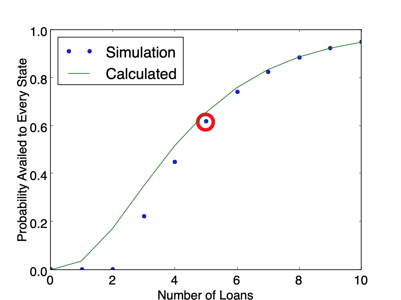
Another Way to Count The Same Thing
Consider the following alternate approach for counting the $5$-loan, $3$-state problem. We will generate the number of lists where the states $A$, $B$, and $C$ show up $2$, $2$, and $1$ times respectively. First, state $A$ can show up in $\binom{5}{2}=10$ of the five locations. Remove the $2$ instances of state A from the list; now state $B$ can show up in $\binom{3}{2}=3$ remaining ways. Once $B$'s locations are picked, there is only one spot remaining for state $C$. Therefore the total number of ways to order this set is $\binom{5}{2}\cdot \binom{3}{2}\cdot \binom{1}{1} = 30$.
The same procedure is computed for all $\binom{4}{2}=6$ partitions of the $5$ states into $3$ non-empty groups in the table below.
| Pattern | Number of Combinations |
|---|---|
| $(1,1,3)$ | $\binom{5}{1}\cdot \binom{4}{1}\cdot \binom{3}{3}=20$ |
| $(1,2,2)$ | $\binom{5}{1}\cdot \binom{4}{2}\cdot \binom{2}{2}=30$ |
| $(1,3,1)$ | $\binom{5}{1}\cdot \binom{4}{1}\cdot \binom{1}{1}=20$ |
| $(2,1,2)$ | $\binom{5}{2}\cdot \binom{3}{1}\cdot \binom{2}{2}=30$ |
| $(2,2,1)$ | $\binom{5}{2}\cdot \binom{3}{2}\cdot \binom{1}{1}=30$ |
| $(3,1,1)$ | $\binom{5}{3}\cdot \binom{2}{1}\cdot \binom{1}{1}=20$ |
This approach affords us a new insight: a clear look at the combinatorial complexity required to count this. We must count the ways to arrange letters for every partition of loans among states. For $5$ loans and $3$ states there are $\binom{4}{2}=6$ partitions, but for $300$ loans and $50$ states there are $\binom{299}{49}=5.19\times 10^{56}$ partitions.
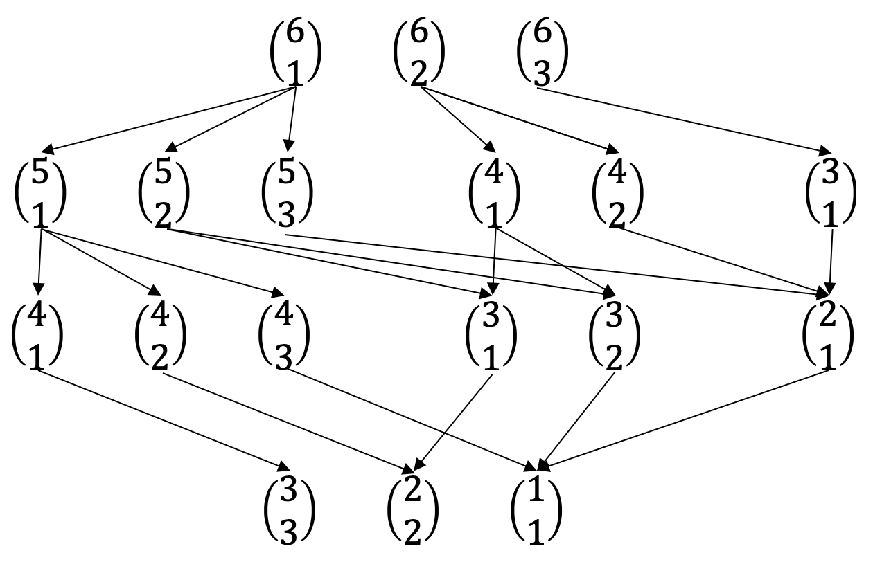
It also affords a nice way to visualize different computations. The $5$-loan, $3$-state problem is a bit bland, but here is a flow chart of the paths to calculate all arrangements for the $6$-loan, $4$-state problem.
The recursive nature of these patterns lends itself to either recursive solutions, or potentially even a dynamic programming algorithm. That said, the simulations were a lot easier to generate and the combinatorial complexity of the problem makes it intractable for large numbers.
Manipulating Res Ipsa
Posted on October 13, 2019
Introduction and Example
A recent torts cases from class (Byrne v. Boadle) served as the introduction to a class of problems where negligence could be considered probabilistically. This set of problems mirrors the more well-known "false positive" problem. Here are two ways to state what is mathematically the same exercise.
"False Positive" problem: A disease afflicts $0.1\%$ of a population. A test exists for the disease, and will show positive $90 \% $ of the time if you have the disease and $1\%$ of the time if you don't (false positive). If you test positive, what is the probability you have the disease?
Negligence problem: Employees of a company act negligently $0.1\%$ of the time they load barrels next to a window. If they act negligently, an accident occurs $90\%$ of the time. When they are not negligent, an accident occurs $1\%$ of the time. If an accident occurs, what is the probability it was due to negligence?
Both have the same solution (we'll use the negligence nomenclature). Define $P_1$, $P_2$, and $P_3$ per the table below.
| Probability | Disease Problem | Negligence Problem |
|---|---|---|
| $P_1=1\%$ | False positive | Accident, not acting negligently |
| $P_2=90\%$ | True positive | Accident, acting negligently |
| $P_3=0.1\%$ | Prevalence of disease | Rate of negligence |
Let's say an accident occurred. The probability an accident occurs through negligence is $P_{negligence}=P_2\cdot P_3=0.00999$. The probability an accident occurs without negligence is $P_{no-negligence}=P_1\cdot(1-P_3) = 0.0009$. Therefore the probability it was due to negligence is: $$ \frac{P_{negligence}}{P_{negligence}+P_{no-negligence}} = 8.3\%.$$ So $8.3\%$ of the time it is due to negligence (or isomorphically, there is an $8.3 \% $ chance you have the disease despite a positive test).
So should this example drive our intuition? Unless this pattern of low rates of negligence holds for a majority of inputs, the answer is a resounding no.
Let's change the problem slightly by making the probability of accident from non-negligence $P_1=0.1\%$ and the rate of negligence $P_3=1\%$. Intuition would tell you negligence is more likely to have been the cause, but by how much? If you work through the same math, the probability the accident was due to negligence now becomes $90.1\%$. Clearly, this problem is susceptible to manipulation through small changes in the inputs.
DIY Inputs
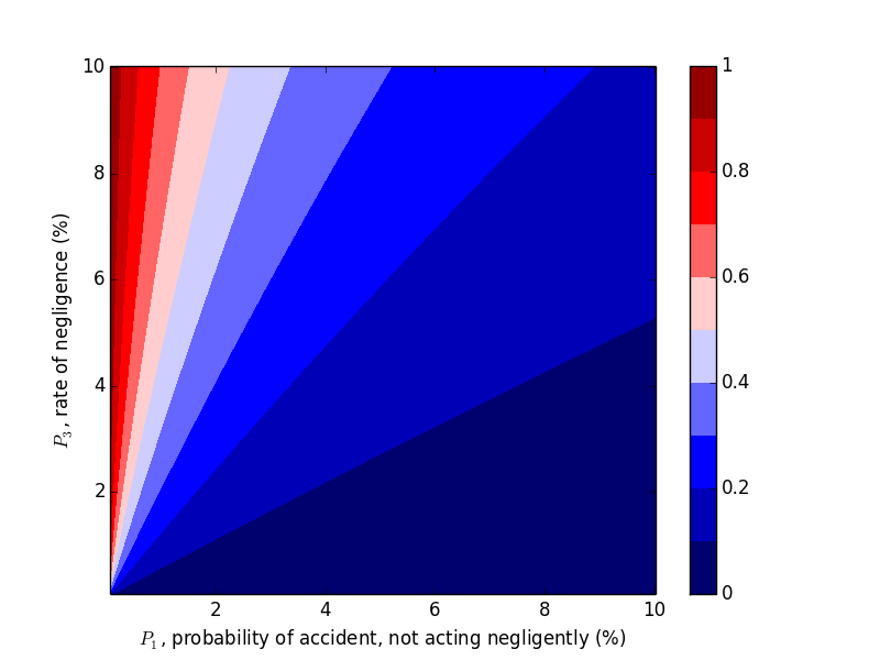
Try a few different cases yourself and see if you can game the outcome. What are the driving variables?Changing $P_1$ and $P_3$
We were able to "flip" the outcome by flipping $P_1$ and $P_3$, so let's look at the probability of negligence as we vary those two variables. Plots can be generated with the following code.
import matplotlib.pyplot as plt

steps = 201
array2d = [range(steps) for _ in range(steps)]

interval = .0005

for i in range(steps):
    for j in range(steps):
        p1 = interval*(i+1)   # probability of drop if properly handled
        p2 = .20              # probability of drop if improperly handled
        p3 = 1-interval*(j+1) # probability of handled properly

        pa = p1*p3            # handled properly but dropped
        pb = (1-p3)*p2        # handled improperly and dropped

        p_proper = pa/(pa+pb)
        array2d[j][i] = p_proper

plt.contourf(array2d, 9, vmin=0.0, vmax=1.0, origin='lower',
             extent=[interval * 100, interval * steps * 100, interval * 100, interval * steps * 100],
             cmap='seismic')

cbar=plt.colorbar()
plt.xlabel('$P_1$, probability of accident, not acting negligently (%)')
plt.ylabel('$P_3$, rate of negligence (%)')
plt.title('Probability that Accident Happened through Negligence, $P_2 = 20\%$')

cbar.set_ticks([0, .2, .4, .6, .8, 1])
cbar.set_ticklabels([0, .2, .4, .6, .8, 1])

plt.show()
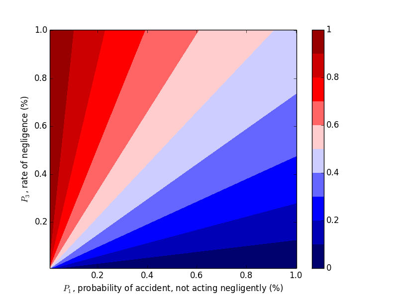
This trend makes sense in hindsight, but one should hardly be expected to carry this intuition around with them, naturally or otherwise.
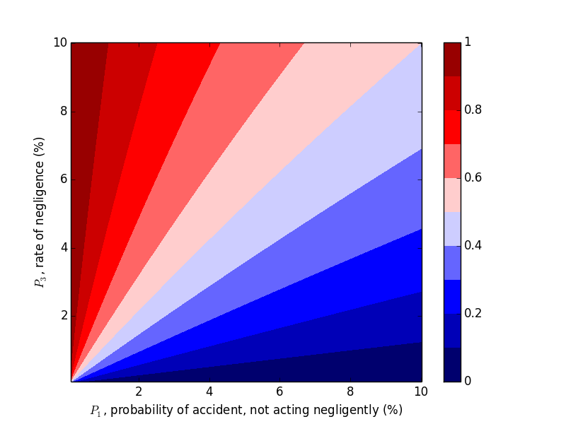
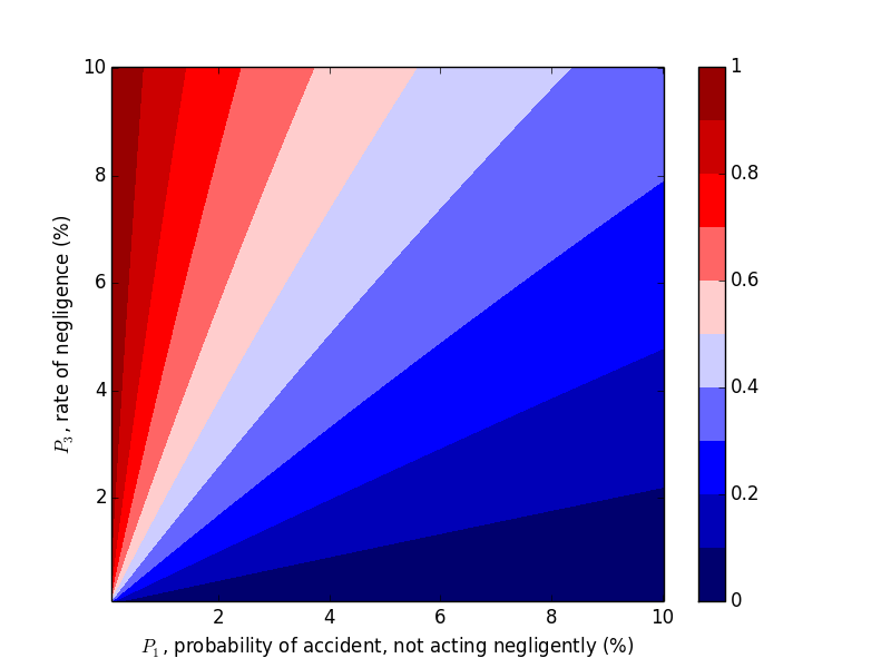
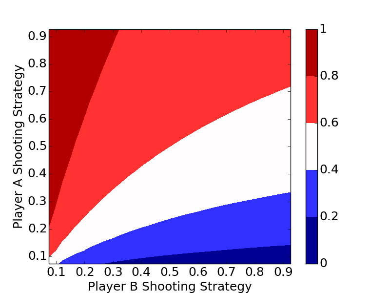
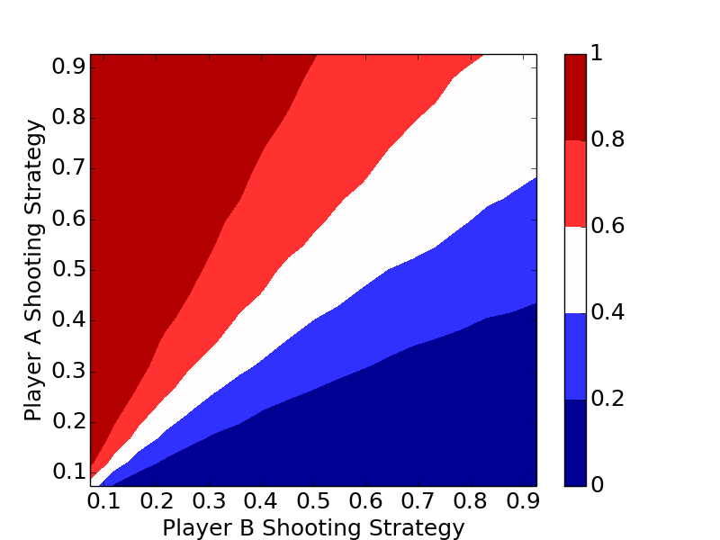
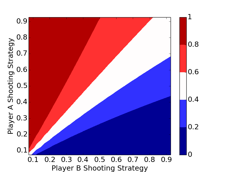
Changing $P_2$
Now let's work with $P_2$. Compare the above plots where $P_2=0.9$ to the plots below where $P_2=0.2, 0.5$. We would expect decreasing $P_2$, probability of an accident given negligence, to decrease the probability of negligence given an accident, which the plots below confirm.
Takeaways
With these results, we can develop a general intuition:
- If $P_2$ is sufficiently low, an accident is probably not due to negligence.
- If $P_2$ is sufficiently high and $P_1>P_3$, then the accident was probably not due to negligence.
- If $P_2$ is sufficiently high and $P_1 < P_3$, then the accident was probably due to negligence.
That said, a more important takeaway here is simpler: don't let a limited data set drive your intuition. Look at the sensitivity of the variables involved, and look at a wide swath of results before jumping to conclusions. And unless you have a clear reason to, don't arbitrarily assume probabilities. You probably don't know the difference between $0.1 \%$ and $1 \%$ without a good data set to aid you.
Optimal HORSE Strategy
Posted on July 14, 2019
Below is a solution to the Classic problem posed on July 12's edition of the Riddler on fivethirtyeight.com, "What’s The Optimal Way To Play HORSE?".
We will first introduce the game, then walk through a simulation, then the analytic solutions for the simplified game of $\mathrm{H}$ then the full game of $\mathrm{HORSE}$. We'll show that the optimal strategy regardless of the number of letters in the game is to always shoot the highest percentage shot (short of a 100% shot).
Intuitive Strategies
Two strategies immediately come mind. First, take a shot that maximizes the probability of you making a basket and him missing.
The second, and provably better strategy is to take advantage of the one thing you have (you are equally good shooters). You get to go first, so take full advantage of that turn, and maximize the probability of scoring a point before you miss.
Intuitive strategies are meaningless unless testing, so let's see what works best.
Simulation and Optimal Strategy
The code below is a bare bones implementation of a simulation. Player A and Player B can be assigned two different strategies, a_prob and b_prob, and the length of the game can be changed.
import random


def make_basket(prob):
    if prob > random.random():
        return True
    else:
        return False


def run_simulation(a_prob, b_prob, horse):
    a_score = 0
    b_score = 0
    a_turn = True

    while True:
        if a_turn:
            if make_basket(a_prob):
                if make_basket(a_prob):
                    pass         # both make
                else:
                    a_score += 1 # a make, b miss
            else:
                a_turn = False   # a misses, it's b's turn

        else:
            if make_basket(b_prob):
                if make_basket(b_prob):
                    pass          # both make
                else:
                    b_score += 1  # b make, a miss
            else:
                a_turn = True     # b misses, it's a's turn

        if a_score >= horse or b_score >= horse:
            break

    return a_score, b_score

The plots clearly show the optimal strategy regardless of the number of letters in the game is to always shoot the highest percentage shot (short of a 100% shot).
Analytic Solution to $\mathrm{H}$
Let's consider the probability of Player A winning a point before losing their turn. Let $a$ be the probability of Player A making a basket. Then they could make a point in two shots with $p_2(a)=a(1-a)$, in four shots with $p_4(a)=a^3(1-a)$, or in general, in $2n$ shots with $p_{2n}(a)=a^{2n-1}(1-a)$. Therefore, the probability $p_A$ of winning a letter before losing their turn is $$p_A=\sum{p_i(a)}=a(1-a)+a^3(1-a)+... = \frac{a(1-a)}{1-a^2}=\frac{a}{a+1}.$$
The maximum value of this function on $[0,1]$ occurs at $a=1$, with $p_A(a)=0.5$. We wouldn't want to shoot a basket neither player ever misses, a trivial solution and never ending game, but we want to pick the shot closest to that.
We'll expand from winning a point without losing a turn, to winning the game of $H$, another geometric sequence. Let the player's probabilities of winning a point without losing a turn be $p_A$ and $p_B$ respectively. Player A could win on the first turn with probability $p_{AH_{1}}=p_A$, on the third turn with probability $p_{AH_{3}}=(1-p_A)(1-p_B)p_A$, and in $2n+1$ turns with probability $$p_{AH_{ 2n+1}}=(1-p_A)^{n}(1-p_B)^np_A$$
Similarly, the probability that Player A wins $H$, $p_{AH}$, is this sum $$p_{AH}=\sum{p_{AH_{2n+1}}}= \frac{p_A}{1-r}.$$ Where $p_A=\displaystyle\frac{a}{a+1}$, $p_B=\displaystyle\frac{b}{b+1}$, and $r=(1-p_A)(1-p_B)$.
As a sanity check, one could sum the terms of the geometric series for the probability of Player B winning, $\displaystyle\frac{(1-p_A)p_B}{1-r}$, add it to the probability of A winning, and find their sum is one, as it should be.
Analytic Solution to $\mathrm{HORSE}$
Expanding to multi-letter games is no longer a game of compounded geometric series, but instead of counting combinations. You can start by thinking of winning $\mathrm{HORSE}$ the same way as winning a five-game series. Unfortunately, it gets a little more complicated; your probability of winning a letter is based off whether or not you won the previous letter.
Let $A$ denote a Player A point win, and $B$ denote a Player B point win. Consider the game $AAAAA$. On each round, Player A starts, so they have the advantage; their probability of winning each point is $P_{AH}$.
Now consider, $ABAAAA$. The Player A win on point 3 following the Player B win, has the lower likelihood $(1-P_{BH})$ of occurring since Player B had the advantage of starting with the ball after winning point 2.
What makes the counting challenging is that the sequences $AABBBAAA$ and $ABABABAA$, for example, do not have the same probabilities for Player A winning. The first only has two "switches" from who is in control (shooting first), where the second has six switches, changing the probabilities in different ways. There is no way around working through each of the individual $1+5+15+35+70=126$ cases for Player A winning in five through nine games respectively.
The code below summarizes this counting.
probs = [.05*i for i in range(1,20)]
for a in probs:
    for b in probs:
        pa = a / (1 + a)
        pb = b / (1 + b)
        r = (1 - pa) * (1 - pb)

        pAH = pa / (1 - r)    # probability a wins going first
        pBH = pb / (1 - r)    # probability b wins going first
        pAB = (1 - pAH, pAH)

        cum_p = 0             # cumulative probability

        for s in ['1111', '01111', '001111', '0001111', '00001111']:
            tups = list(perm_unique(s))
            for tup in tups:
                seq = [int(i) for i in list(tup)+['1']]

                p = pAB[seq[0]]
                for i in range(1, len(seq)):
                    if seq[i-1] == 0 and seq[i] == 0:
                        p *= pBH
                    elif seq[i-1] == 1 and seq[i] == 0:
                        p *= (1 - pAH)
                    elif seq[i-1] == 0 and seq[i] == 1:
                        p *= (1 - pBH)
                    elif seq[i-1] == 1 and seq[i] == 1:
                        p *= pAH
                cum_p += p
        print cum_p,
    print ""
My code makes use of some StackOverflow code to make unique permutations.
Winning Lotería and Countdown
Posted on June 2, 2019
Updated on June 4, 2019
I made a few changes from the original post. I misread allowable order of operations (the equivalent of "parentheses are ok", which drastically increases solvable numbers). I decided to leave it in as an interesting twist on the problem.
I also left out the case of six small numbers (another misread), which I have since added.
Below are solutions to the Classic and Express problems posed on May 31's edition of the Riddler on fivethirtyeight.com, "Can You Win The Lotería?".
Riddler Express - Lotería
First, a brief solution to the Riddler Express. The question posed is: for $N=54$ total images, and $n=16$ images per player card, how often will the game end with one empty card of images?
Two things must be considered: how often do the two players have unique cards (a necessary condition), and if that is met, how often will an entire card be filled before any images on the second card are filled?
We must first consider the necessary condition that the players have unique images on their cards. It helps to think about image "selection" successively. The first player can pick their entire card without concern. Then the second player "picks" their images for the second card one by one. For $N=54$ and $n=16$, there are $54$ options, $54-16=38$ of which are favorable, so probability the first image for the second card is not on the first card is $\frac{38}{54}$. The second image cannot be the first (and will not be the previous image), so there are now $53$ options, $37$ of which are favorable, yielding a probability of $\frac{37}{53}$. Continuing this logic, the probability the cards are unique is
$$ \frac{38}{54}\cdot\frac{37}{53}\cdot\frac{36}{52}\cdot...\cdot\frac{23}{39} \approx 0.001054.$$In general, the probability can be written as
$$ \displaystyle\frac{\binom{N-n}{n}}{\binom{N}{n}}.$$ Second, assuming the two cards are unique, how often will you win before the other player crosses a single image off their card? The extraneous cards are meaningless, akin to burn cards. WLOG, if you have images $1$-$16$, your opponent has $17$-$32$, then the favorable outcomes are all $16!$ arrangements of your cards, followed by all $16!$ arrangements of your opponents outcomes. The total number of arrangements is $32!$, the arrangements of all cards. The probability is then $$ \displaystyle\frac{16!\cdot 16!}{32!} \approx 1.664\times 10^{-9}. $$In general, the probability can be written as
$$ \displaystyle\frac{(n!)^2}{(2n)!}. $$Note, there is no $N$ term in this expression. The simulation in the code below considers all $N$ cards to verify its invariance.
from ncr import ncr #n choose r
import numpy as np


def you_win(photo_order, n):
    """WLOG you have photos 0 to n-1, opponent has n to 2n-1
    Check if all of your photos appear before any of your opponents"""
    n_count = 0
    for i in photo_order:
        if i < n:
            n_count += 1
        if n <= i < 2*n:
            return False
        if n_count == n:
            return True


def main():
    N = 54          # Total number of photos
    n = 16          # Number of photos per player
    num_sim = 10000 # Number of simulations

    # Simulate Unique
    count = 0
    for _ in xrange(num_sim):
        list_1 = np.random.choice(N, n, replace=False) # Your photos
        list_2 = np.random.choice(N, n, replace=False) # Opponent's photos
        if set(list_1) & set(list_2): # Check for intersection
            count += 1
    print "probability unique:", \
        ncr(N-n, n) / float(ncr(N, n)), \
        1.0 - count / float(num_sim)

    # Simulate You Win
    count = 0
    for _ in xrange(num_sim):
        photo_order = np.arange(N)
        np.random.shuffle(photo_order)
        if you_win(photo_order, n):
            count += 1
    print "probability you win:", 1./ncr(2 * n, n), count / float(num_sim)


if __name__ == "__main__":
    main()
Riddler Classic - Countdown
$\newcommand{\Lone}{\mathrm{L}_{1}}$ $\newcommand{\Ltwo}{\mathrm{L}_{2}}$ $\newcommand{\Lthree}{\mathrm{L}_{3}}$ $\newcommand{\Lfour}{\mathrm{L}_{4}}$ $\newcommand{\a}{\mathrm{a}}$ $\newcommand{\b}{\mathrm{b}}$ $\newcommand{\c}{\mathrm{c}}$ $\newcommand{\d}{\mathrm{d}}$ $\newcommand{\e}{\mathrm{e}}$The remainder of this post will focus on the countdown problem, namely a brute force approach to counting all possible outcomes in a reasonable amount of time, follwed by a discussion of results. See code here.
The most fruitful combination is shown to be $5$, $6$, $8$, $9$, $75$, $100$, which yields $691$ different three-digit numbers. The least fruitful is shown to be $1$, $1$, $2$, $2$, $3$, $25$, which yields only $20$ different three-digit numbers.
Statistics for the various strategies (selecting 1 through 4 large numbers) are summarized, and it is shown that selecting two large numbers is the most advantageous, followed closely by selecting three large numbers.
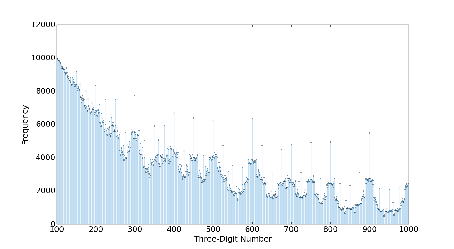
Finally, a histogram of the three-digit numbers frequency among the $10,603$ combinations shows what is intuitive, at least in hindsight: smaller three-digit numbers, and multiples of $25$, $50$, and especially $100$ are the most common.
Generating Combinations
First we must consider all possible combinations of the small and large numbers. We will denote large numbers with $\Lone$, $\Ltwo$, $\Lthree$, and $\Lfour$ and small numbers with $\a$, $\b$, $\c$, $\d$ and $\e$. A player can selected between zero and four large numbers, and the small numbers may repeat once. There are $11$ possible scenarios, divided by double lines in the table below by strategy.
| Pattern | Number of Combinations |
|---|---|
| $\a\b\c\d\e\mathrm{f}$ | $\binom{10}{6}$ |
| $\Lone\a\a\b\b\c$ | $\binom{4}{1}\cdot\binom{10}{2}\cdot\binom{8}{1}$ |
| $\Lone\a\a\b\c\d$ | $\binom{4}{1}\cdot\binom{10}{1}\cdot\binom{9}{3}$ |
| $\Lone\a\b\c\d\e$ | $\binom{4}{1}\cdot\binom{10}{5}$ |
| $\Lone\Ltwo\a\a\b\b$ | $\binom{4}{2}\cdot\binom{10}{2}$ |
| $\Lone\Ltwo\a\a\b\c$ | $\binom{4}{2}\cdot\binom{10}{2}\cdot\binom{8}{1}$ |
| $\Lone\Ltwo\a\b\c\d$ | $\binom{4}{2}\cdot\binom{10}{4}$ |
| $\Lone\Ltwo\Lthree\a\a\b$ | $\binom{4}{3}\cdot \binom{10}{1}\cdot \binom{9}{1}$ |
| $\Lone\Ltwo\Lthree\a\b\c$ | $\binom{4}{3}\cdot\binom{10}{3}$ |
| $\Lone\Ltwo\Lthree\Lfour\a\a$ | $\binom{4}{4}\cdot\binom{10}{1}$ |
| $\Lone\Ltwo\Lthree\Lfour\a\b$ | $\binom{4}{4}\cdot\binom{10}{2}$ |
Generating Permutations
These can be generated individually with the help of the Python itertools library. As a sample, consider $\Lone\Ltwo\a\a\b\c$.
import itertools
L_array = [25., 50., 75., 100.]
s_array = [float(i) for i in range(1, 11)]

for s in itertools.combinations(s_array, 3):
    for L in itertools.combinations(L_array, 2):
        for s0 in s:
            loop_array = itertools.permutations(list(L) + list(s) + [s0])
This is probably the most complicated of the $11$ examples. Note the use of itertools.combinations vs itertools.permutations, the latter provides all arrangements and the former does not, which helps us reduce over counting. Over counting is not completely avoided however. The itertools library does not know that our two $\a$ values are repeats so we are over counting by a factor of $2$. This is not ideal, but the storage mechanism used (based on Python sets and dicts) eliminates error duplicate counting, so the only sacrifice is run time.
Considering Operators: $+-\times\div$
We will now take each permutation generated and loop through it's components left to right (i.e. consider the first number, then the first two numbers, then the first three, etc.). For example, given the permutation $100$, $50$, $10$, $2$, $7$, $4$, the first number "generated" is $100$. We then need to check all operations with the first two terms, $100+50$, $100-50$, $100\times 50$, and $100\div 50$ which yields $150$, another hit, but three numbers, $50$, $5000$, and $2$ that are not hits. Those last three numbers are not hits, but cannot be ignored since additional terms may turn them into hits; for example $100\times 50\div 10\div 2=250$ is another hit.
Challenges also arise with the implementation of addition, subtraction, multiplication and division operations in this left-to-right paradigm. We have $5$ spaces in between the $6$ numbers for each operation, for $4^5=1024$ possible permutations of the operators. However, we must only consider those where left to right operation satisfies order of operations. For example, $+$ $-$ $+$ $-$ $-$, $\div$ $\times$ $\div$ $\times$ $\div$, and $\times$ $\div$ $-$ $-$ $+$ are all acceptable but $+$ $\times$ $-$ $-$ $-$ because placing addition before multiplication is the equivalent of adding parentheses. Using the above example, $100+50+10\times2$
Acceptable orders of operation can be found with the following code. This finds all lists of five operators where all multiplication and division occur before all addition and subtraction.
operator_list = [] # Indices for operators, 0,1,2,3 is *,/,+,-
for i4 in xrange(4 ** 5):
    cl = [i4 // 256 % 4, i4 // 64 % 4, i4 // 16 % 4, i4 // 4 % 4, i4 % 4]
    if good_order(cl):
        operator_list.append(cl)
print len(operator_list) # 192
Proving that this covers every possible case is not simple, but it makes intuitive sense that when all permutations of the 6 numbers are considered, the $192$ operators considered are exhaustive.
We now have everything we need to search for every combination. Full implementation can be found here.
A Brief Summary of Results
The combination $5$, $6$, $8$, $9$, $75$, $100$, yields $691$ different possible three-digit numbers, the most for any combination. The combination $1$, $1$, $2$, $2$, $3$, $25$, yields only $20$ possible combinations, the fewest. The top and bottom ten combinations are summarized in the tables below.
| Number | Number of three-digit numbers created |
|---|---|
| $5$, $6$, $8$, $9$, $75$, $100$ | $691$ |
| $5$, $7$, $8$, $9$, $75$, $100$ | $652$ |
| $6$, $7$, $9$, $10$, $75$, $100$ | $650$ |
| $6$, $8$, $9$, $10$, $75$, $100$ | $648$ |
| $3$, $8$, $9$, $10$, $75$, $100$ | $648$ |
| $2$, $5$, $6$, $9$, $75$, $100$ | $643$ |
| $5$, $6$, $8$, $9$, $50$, $100$ | $641$ |
| $5$, $6$, $7$, $9$, $75$, $100$ | $640$ |
| $2$, $5$, $8$, $9$, $75$, $100$ | $638$ |
| $4$, $7$, $9$, $10$, $75$, $100$ | $636$ |
| Number | Number of three-digit numbers created |
|---|---|
| $1$, $1$, $2$, $2$, $3$, $25$ | $20$ |
| $1$, $1$, $2$, $2$, $4$, $25$ | $21$ |
| $1$, $1$, $2$, $3$, $3$, $25$ | $25$ |
| $1$, $1$, $3$, $4$, $4$, $25$ | $34$ |
| $1$, $1$, $2$, $2$, $6$, $25$ | $35$ |
| $1$, $1$, $2$, $2$, $9$, $25$ | $35$ |
| $1$, $1$, $2$, $2$, $5$, $25$ | $35$ |
| $1$, $1$, $2$, $2$, $7$, $25$ | $35$ |
| $1$, $1$, $2$, $2$, $4$, $50$ | $36$ |
| $1$, $1$, $2$, $4$, $4$, $25$ | $36$ |
The table below shows that the best choice to pick two large numbers and four small numbers, but the strategy of picking three large is a close second. An outcome is defined as a three-digit number generated by a particular combination.
| Pattern | Arrangements | Total Outcomes | Average # of Outcomes |
|---|---|---|---|
| $\a\b\c\d\e\mathrm{f}$ | $210$ | $46,663$ | $222.2$ |
| $\Lone\a\a\b\b\c$ | $1440$ | $257,167$ | $178.6$ |
| $\Lone\a\a\b\c\d$ | $3360$ | $865,253$ | $257.5$ |
| $\Lone\a\b\c\d\e$ | $1008$ | $349,921$ | $347.1$ |
| One large | $253.5$ | ||
| $\Lone\Ltwo\a\a\b\b$ | $270$ | $58,221$ | $215.6$ |
| $\Lone\Ltwo\a\a\b\c$ | $2160$ | $694,966$ | $321.7$ |
| $\Lone\Ltwo\a\b\c\d$ | $1260$ | $574,520$ | $456.0$ |
| Two large | $\pmb{359.8}$ | ||
| $\Lone\Ltwo\Lthree\a\a\b$ | $360$ | $100,324$ | $278.7$ |
| $\Lone\Ltwo\Lthree\a\b\c$ | $480$ | $199,349$ | $415.3$ |
| Three large | $356.8$ | ||
| $\Lone\Ltwo\Lthree\Lfour\a\a$ | $10$ | $1,541$ | $154.1$ |
| $\Lone\Ltwo\Lthree\Lfour\a\b$ | $45$ | $10,619$ | $236.0$ |
| Four large | $221.1$ |
The histogram shows what we would intuitively expect, smaller numbers can be computed more often. There are also peaks at multiples of $25$, $50$, and especially $100$, another intuitive byproduct.
Flipping Astronauts
Posted on May 26, 2019
Introduction
This is a solution to the problem posed on May 24's edition of the Riddler Classic on fivethirtyeight.com, "One Small Step For Man, One Giant Coin Flip For Mankind".
We will show that there are $12$ non-trivial solutions to the $3$-astronaut problem with $4$ coins and $2$ non-trivial solutions to the $5$-astronaut problem with $6$ coins.
Three Astronauts
The problem statement walks through the impossibility of using two coins, with $2^2=4$ outcomes, to determine a winner for three astronauts. The same can be said for three flips, which we will briefly discuss.
The key to attacking this problem for an $n$-astronaut scenario is equally distributing outcomes amongst the first $n-1$ astronauts. For the $3$-astronaut, $3$-flip case this translates to the following: among the $1$, $3$, $3$, and $1$ outcomes ($0$ heads, $1$ head, $2$ heads, and $3$ heads respectively), the first and second astronauts should have the same number each of $0$-head, $1$-head, $2$-head, and $3$-head outcomes. One possible assignment that meets this parameter is for the first and second astronauts to each have the distributions $0$, $1$, $1$, $0$, leaving the third astronaut with the distribution $1$, $1$, $1$, $1$. This is summarized in the table, below.
| 3 Heads 0 Tails | 2 Heads 1 Tail | 1 Head 2 Tails | 0 Heads 3 Tails |
|
|---|---|---|---|---|
| Astro #1 | 0 | 1 | 1 | 0 |
| Astro #2 | 0 | 1 | 1 | 0 |
| Astro #3 | 1 | 1 | 1 | 1 |
| Total | 1 | 3 | 3 | 1 |
This distribution, however, implies that the probability of flipping three heads and zero heads is both zero, a contradiction. All distributions with $3$ astronauts and $3$ coins yield similar contradictions.
There is no rigorous proof here to the claim that the first $n-1$ astronauts must have the same distribution of outcomes, but the likelihood of them having different outcomes that independently add up to a very specific fraction is highly unlikely. Further work below will show it's analogous to polynomials with different integer coefficients having an identical real root between $0$ and $1$.
We broaden our horizons to a $4$-coin solution, which has the $2^4=16$ outcomes of $1$, $4$, $6$, $4$, $1$, for $4$, $3$, $2$, $1$, and $0$ heads respectively. For three astronauts, we have significantly more ways to distribute the coin flips. For example, the first two astronauts could each be given the outcome distribution $0$, $2$, $3$, $2$, $0$, leaving $1$, $0$, $0$, $0$, $1$ for the third astronaut. This is summarized in the table, below.
| 4 Heads 0 Tails | 3 Heads 1 Tail | 2 Heads 2 Tails | 1 Head 3 Tails | 0 Heads 4 Tails |
|
|---|---|---|---|---|---|
| Astro #1 | 0 | 2 | 3 | 2 | 0 |
| Astro #2 | 0 | 2 | 3 | 2 | 0 |
| Astro #3 | 1 | 0 | 0 | 0 | 1 |
| Total | 1 | 4 | 6 | 4 | 1 |
We now have to see if a solution exists with this distribution. Let $h$ be the probability of flipping a heads, and $t=1-h$ be the probability of flipping a tails. We generate the probabilities of each flipping outcome: for $k$ heads in $n$ flips, a specific outcome (ignoring rearrangments) is $h^k t^{n-k} = h^k (1-h)^{n-k}$. Using the current example from the above table, our probability polynomial for astronaut 1 (and equivalently astronaut 2) becomes
\begin{eqnarray} 2 h^3 (1-h) + 3 h^2 (1-h)^2 + 2 h (1-h)^3 &=& \frac{1}{3} \\ -h^4 + 2h^3 -3 h^2 + 2h &=& \frac{1}{3} \end{eqnarray} $$ h = \frac{1}{6} \left( 3 \pm \sqrt{3 \left(4\sqrt{6} -9\right)} \right) \approx 0.242, 0.758 $$Therefore, we can state that one solution is with $h=.242$, the first astronaut getting assigned $2$, $3$, and $2$ each of the $3$-head, $2$-head, and $1$-head outcomes, and the third astronaut being assigned the $4$-head and $0$-head outcomes.
As an aside, it makes sense to have symmetric solutions here (that is, they add up to $1$), since we picked symmetric coefficients $2$, $3$, and $2$. We expect an asymmetric pick like $1$, $3$, $2$ to not yield symmetric solutions.
Let's generalize further to find all $3$-astronaut, $4$-coin solutions. There are $4$ outcomes with $3$ heads, so astronauts one and two could each get $0$, $1$, or $2$. Similarly they could get $0$, $1$, $2$, or $3$ and $0$, $1$, or $2$ of the $2$-head outcomes and $1$-head outcomes respectively. We need to test all of these scenarios, which we accomplish using the following code.
import numpy as np
import operator as op
from functools import reduce
from collections import namedtuple

Solution = namedtuple('Solution', 'coefficients roots')


def ncr(n, r):
    """Implementation of n choose r = n!/(r!*(n-r)!)"""
    r = min(r, n-r)
    numer = reduce(op.mul, range(n, n-r, -1), 1)
    denom = reduce(op.mul, range(1, r+1), 1)
    return numer / denom


def create_polys(num_coins):
    """Creates polynomial expansions in list form for n-1 to 1 heads"""
    polys = []
    for i in range(1, num_coins):
        poly = []
        neg = (-1)**i
        for j in range(0, i+1):
            poly.append(ncr(i, j) * neg)
            neg *= -1
        for k in range(i+1, num_coins):
            poly.append(0)

        polys.append(poly)
    return polys


def create_coeff_limits(num_coins, num_astronauts):
    """Determines the maximum allocation of head/tail outcomes based off the number of coins and astronauts"""
    coeffs = []
    for i in range(1, num_coins):
        coeffs.append(ncr(num_coins, i) // (num_astronauts - 1) + 1)
    return coeffs


def is_valid_solution(root):
    """Checks if root is valid.  Must be real and between 0 and 1."""
    return np.isreal(root) and 0 < root < 1


def solve_poly(coeffs, polys, prob):
    """Generates and solves polynomials using np.roots
    coeffs: list of "coefficients", i.e. multipliers for the number of out head/tail outcomes
    polys: generated with create_polys
    prob: the negated probability -1/num_astronauts
    returns all valid solutions a list on named tuples
    """
    sum_poly = []
    valid_solutions = []
    for degree in range(len(polys[0])):
        term = 0
        for j in range(len(polys)):  # for each polynomial
            term += coeffs[j] * polys[j][degree]
        sum_poly.append(term)
    sum_poly.append(prob)
    ans = np.roots(sum_poly)
    for root in ans:
        if is_valid_solution(root):
            valid_solutions.append(Solution(coeffs, root))

    return valid_solutions


def main():
    num_astronauts = 3
    num_coins = 6
    prob = -1.0/num_astronauts
    polys = create_polys(num_coins)
    coeff_limits = create_coeff_limits(num_coins, num_astronauts)
    solutions = []

    # Loop through all possible coefficient combinations
    coeff_dividers = []
    for i in range(1, len(coeff_limits)):
        coeff_dividers.append(reduce(op.mul, coeff_limits[i:], 1))

    # This helps us avoid recursion and nested for loops
    for i in range(reduce(op.mul, coeff_limits, 1)):
        coeffs = []
        for j in range(len(coeff_dividers)):
            coeffs.append((i // coeff_dividers[j]) % coeff_limits[j])
        coeffs.append(i % coeff_limits[-1])
        solutions += solve_poly(coeffs, polys, prob)

    for solution in solutions:
        print solution.coefficients, np.real(solution.roots) #strip 0.j
    print "Number of solutions:", len(solutions)


if __name__ == '__main__':
    main()
This code, with num_astronauts=3 and num_coins=4 yields the following 12 solutions, where the five listed values correspond to distributions with $4$, $3$, $2$, $1$, and $0$ heads respectively.
| $h$ | Astronauts 1 & 2 | Astronaut 3 |
|---|---|---|
| 0.4505 | 0, 0, 3, 2, 0 | 1, 4, 0, 0, 1 |
| 0.2861 | 0, 0, 3, 2, 0 | 1, 4, 0, 0, 1 |
| 0.6051 | 0, 1, 3, 2, 0 | 1, 2, 0, 0, 1 |
| 0.2578 | 0, 1, 3, 2, 0 | 1, 2, 0, 0, 1 |
| 0.6967 | 0, 2, 2, 2, 0 | 1, 0, 2, 0, 1 |
| 0.3033 | 0, 2, 2, 2, 0 | 1, 0, 2, 0, 1 |
| 0.7139 | 0, 2, 3, 0, 0 | 1, 0, 0, 4, 1 |
| 0.5495 | 0, 2, 3, 0, 0 | 1, 0, 0, 4, 1 |
| 0.7422 | 0, 2, 3, 1, 0 | 1, 0, 0, 2, 1 |
| 0.3949 | 0, 2, 3, 1, 0 | 1, 0, 0, 2, 1 |
| 0.7579 | 0, 2, 3, 2, 0 | 1, 0, 0, 0, 1 |
| 0.2421 | 0, 2, 3, 2, 0 | 1, 0, 0, 0, 1 |
Five Astronauts
The problem is easily generalized with the above code to higher numbers of astronauts. There are two solutions for $5$ astronauts and $6$ coins, where the seven listed values correspond to distributions with $6$, $5$, $4$, $3$, $2$, $1$, and $0$ heads respectively.
| $h$ | Astronauts 1, 2, 3, & 4 | Astronaut 5 |
|---|---|---|
| 0.4326 | 0, 1, 3, 5, 3, 1, 0 | 1, 2, 3, 0, 3, 2, 1 |
| 0.5674 | 0, 1, 3, 5, 3, 1, 0 | 1, 2, 3, 0, 3, 2, 1 |
We can also search for solutions with larger numbers of coins. The $64$ solutions for $5$ astronauts and $7$ coins are listed in the table below, where the eight listed values correspond to distributions with $7$, $6$, $5$, $4$, $3$, $2$, $1$, and $0$ heads respectively.
| $h$ | Astronauts 1, 2, 3, & 4 | Astronaut 5 |
|---|---|---|
| 0.4662 | 0, 0, 3, 8, 8, 5, 1, 0 | 1, 7, 9, 3, 3, 1, 3, 1 |
| 0.3636 | 0, 0, 3, 8, 8, 5, 1, 0 | 1, 7, 9, 3, 3, 1, 3, 1 |
| 0.4536 | 0, 0, 4, 7, 8, 5, 1, 0 | 1, 7, 5, 7, 3, 1, 3, 1 |
| 0.3863 | 0, 0, 4, 7, 8, 5, 1, 0 | 1, 7, 5, 7, 3, 1, 3, 1 |
| 0.5215 | 0, 0, 4, 8, 8, 5, 1, 0 | 1, 7, 5, 3, 3, 1, 3, 1 |
| 0.3468 | 0, 0, 4, 8, 8, 5, 1, 0 | 1, 7, 5, 3, 3, 1, 3, 1 |
| 0.527 | 0, 0, 5, 7, 8, 5, 1, 0 | 1, 7, 1, 7, 3, 1, 3, 1 |
| 0.359 | 0, 0, 5, 7, 8, 5, 1, 0 | 1, 7, 1, 7, 3, 1, 3, 1 |
| 0.5343 | 0, 0, 5, 8, 7, 5, 1, 0 | 1, 7, 1, 3, 7, 1, 3, 1 |
| 0.3845 | 0, 0, 5, 8, 7, 5, 1, 0 | 1, 7, 1, 3, 7, 1, 3, 1 |
| 0.543 | 0, 0, 5, 8, 8, 4, 1, 0 | 1, 7, 1, 3, 3, 5, 3, 1 |
| 0.4207 | 0, 0, 5, 8, 8, 4, 1, 0 | 1, 7, 1, 3, 3, 5, 3, 1 |
| 0.5513 | 0, 0, 5, 8, 8, 5, 0, 0 | 1, 7, 1, 3, 3, 1, 7, 1 |
| 0.4487 | 0, 0, 5, 8, 8, 5, 0, 0 | 1, 7, 1, 3, 3, 1, 7, 1 |
| 0.5742 | 0, 0, 5, 8, 8, 5, 1, 0 | 1, 7, 1, 3, 3, 1, 3, 1 |
| 0.3363 | 0, 0, 5, 8, 8, 5, 1, 0 | 1, 7, 1, 3, 3, 1, 3, 1 |
| 0.4564 | 0, 1, 2, 8, 8, 5, 1, 0 | 1, 3, 13, 3, 3, 1, 3, 1 |
| 0.3758 | 0, 1, 2, 8, 8, 5, 1, 0 | 1, 3, 13, 3, 3, 1, 3, 1 |
| 0.5278 | 0, 1, 3, 8, 8, 5, 1, 0 | 1, 3, 9, 3, 3, 1, 3, 1 |
| 0.3532 | 0, 1, 3, 8, 8, 5, 1, 0 | 1, 3, 9, 3, 3, 1, 3, 1 |
| 0.5376 | 0, 1, 4, 7, 8, 5, 1, 0 | 1, 3, 5, 7, 3, 1, 3, 1 |
| 0.3673 | 0, 1, 4, 7, 8, 5, 1, 0 | 1, 3, 5, 7, 3, 1, 3, 1 |
| 0.5519 | 0, 1, 4, 8, 7, 5, 1, 0 | 1, 3, 5, 3, 7, 1, 3, 1 |
| 0.396 | 0, 1, 4, 8, 7, 5, 1, 0 | 1, 3, 5, 3, 7, 1, 3, 1 |
| 0.5674 | 0, 1, 4, 8, 8, 4, 1, 0 | 1, 3, 5, 3, 3, 5, 3, 1 |
| 0.4326 | 0, 1, 4, 8, 8, 4, 1, 0 | 1, 3, 5, 3, 3, 5, 3, 1 |
| 0.5793 | 0, 1, 4, 8, 8, 5, 0, 0 | 1, 3, 5, 3, 3, 1, 7, 1 |
| 0.457 | 0, 1, 4, 8, 8, 5, 0, 0 | 1, 3, 5, 3, 3, 1, 7, 1 |
| 0.5995 | 0, 1, 4, 8, 8, 5, 1, 0 | 1, 3, 5, 3, 3, 1, 3, 1 |
| 0.3409 | 0, 1, 4, 8, 8, 5, 1, 0 | 1, 3, 5, 3, 3, 1, 3, 1 |
| 0.5566 | 0, 1, 5, 6, 8, 5, 1, 0 | 1, 3, 1, 11, 3, 1, 3, 1 |
| 0.3849 | 0, 1, 5, 6, 8, 5, 1, 0 | 1, 3, 1, 11, 3, 1, 3, 1 |
| 0.5831 | 0, 1, 5, 7, 7, 5, 1, 0 | 1, 3, 1, 7, 7, 1, 3, 1 |
| 0.4169 | 0, 1, 5, 7, 7, 5, 1, 0 | 1, 3, 1, 7, 7, 1, 3, 1 |
| 0.604 | 0, 1, 5, 7, 8, 4, 1, 0 | 1, 3, 1, 7, 3, 5, 3, 1 |
| 0.4481 | 0, 1, 5, 7, 8, 4, 1, 0 | 1, 3, 1, 7, 3, 5, 3, 1 |
| 0.6155 | 0, 1, 5, 7, 8, 5, 0, 0 | 1, 3, 1, 7, 3, 1, 7, 1 |
| 0.4657 | 0, 1, 5, 7, 8, 5, 0, 0 | 1, 3, 1, 7, 3, 1, 7, 1 |
| 0.6287 | 0, 1, 5, 7, 8, 5, 1, 0 | 1, 3, 1, 7, 3, 1, 3, 1 |
| 0.351 | 0, 1, 5, 7, 8, 5, 1, 0 | 1, 3, 1, 7, 3, 1, 3, 1 |
| 0.6151 | 0, 1, 5, 8, 6, 5, 1, 0 | 1, 3, 1, 3, 11, 1, 3, 1 |
| 0.4434 | 0, 1, 5, 8, 6, 5, 1, 0 | 1, 3, 1, 3, 11, 1, 3, 1 |
| 0.6137 | 0, 1, 5, 8, 7, 4, 0, 0 | 1, 3, 1, 3, 7, 5, 7, 1 |
| 0.5464 | 0, 1, 5, 8, 7, 4, 0, 0 | 1, 3, 1, 3, 7, 5, 7, 1 |
| 0.6327 | 0, 1, 5, 8, 7, 4, 1, 0 | 1, 3, 1, 3, 7, 5, 3, 1 |
| 0.4624 | 0, 1, 5, 8, 7, 4, 1, 0 | 1, 3, 1, 3, 7, 5, 3, 1 |
| 0.641 | 0, 1, 5, 8, 7, 5, 0, 0 | 1, 3, 1, 3, 7, 1, 7, 1 |
| 0.473 | 0, 1, 5, 8, 7, 5, 0, 0 | 1, 3, 1, 3, 7, 1, 7, 1 |
| 0.649 | 0, 1, 5, 8, 7, 5, 1, 0 | 1, 3, 1, 3, 7, 1, 3, 1 |
| 0.3713 | 0, 1, 5, 8, 7, 5, 1, 0 | 1, 3, 1, 3, 7, 1, 3, 1 |
| 0.6242 | 0, 1, 5, 8, 8, 2, 1, 0 | 1, 3, 1, 3, 3, 13, 3, 1 |
| 0.5436 | 0, 1, 5, 8, 8, 2, 1, 0 | 1, 3, 1, 3, 3, 13, 3, 1 |
| 0.6364 | 0, 1, 5, 8, 8, 3, 0, 0 | 1, 3, 1, 3, 3, 9, 7, 1 |
| 0.5338 | 0, 1, 5, 8, 8, 3, 0, 0 | 1, 3, 1, 3, 3, 9, 7, 1 |
| 0.6468 | 0, 1, 5, 8, 8, 3, 1, 0 | 1, 3, 1, 3, 3, 9, 3, 1 |
| 0.4722 | 0, 1, 5, 8, 8, 3, 1, 0 | 1, 3, 1, 3, 3, 9, 3, 1 |
| 0.6532 | 0, 1, 5, 8, 8, 4, 0, 0 | 1, 3, 1, 3, 3, 5, 7, 1 |
| 0.4785 | 0, 1, 5, 8, 8, 4, 0, 0 | 1, 3, 1, 3, 3, 5, 7, 1 |
| 0.6591 | 0, 1, 5, 8, 8, 4, 1, 0 | 1, 3, 1, 3, 3, 5, 3, 1 |
| 0.4005 | 0, 1, 5, 8, 8, 4, 1, 0 | 1, 3, 1, 3, 3, 5, 3, 1 |
| 0.6637 | 0, 1, 5, 8, 8, 5, 0, 0 | 1, 3, 1, 3, 3, 1, 7, 1 |
| 0.4258 | 0, 1, 5, 8, 8, 5, 0, 0 | 1, 3, 1, 3, 3, 1, 7, 1 |
| 0.6678 | 0, 1, 5, 8, 8, 5, 1, 0 | 1, 3, 1, 3, 3, 1, 3, 1 |
| 0.3322 | 0, 1, 5, 8, 8, 5, 1, 0 | 1, 3, 1, 3, 3, 1, 3, 1 |
Bonus: Riddler Express
The code below is an brute-force solution to the Riddler Express problem about soccer team selection. The smallest solution found was with jersey numbers $1$, $5$, $6$, $8$, $9$, $10$, $12$, $15$, $18$, $20$, and $24$.
import itertools

def brute_soccer(team_list):
    average_score = sum([1./i for i in team_list])
    if abs(average_score-2.0) < 1e-8:
        print team_list, average_score

for i in itertools.combinations(range(1, 25), 11):
    brute_soccer(i)
Efficient Item Swapping Between Nodes
Posted on April 9, 2019
Introduction
A new uniform is coming to the Air Force: the OCP (Operational Camouflage Pattern) is replacing the ABU (Airmen Battle Uniform). Despite the long-term simplicity and cost savings that stem from the Air Force and Army sharing a common uniform, a number of short-term challenges arise.
As part of the ABU's retirement, the 145 Air Force ROTC detachments across the country are being asked to trade uniform items among themselves in lieu of making new purchases, an admirable cost-saving, waste-reducing goal. So, for example, if Det 002 has three extra 'Mens 38L ABU Blouse', and Det 075 needs three of them, Det 002 could ship those three blouses to Det 075. If there were just a few items or few detachments, this exercise would be trivial. However, many detachments need hundreds of uniform items 400+ distinct uniform item types spread among the 145 detachments. The complexity grows quickly.
Given a set number of total swaps (shipments), maximize the number of transferred items (uniforms) between nodes (detachments)
A (notional) detachment may need as many 100 items from (say) 30 item types, maybe only 90 of which can be provided by other dets, and it may required shipments from (say) 7 of those detachments. If this were the case, then hundreds of shipments need to be coordinated on dynamically changing information (every shipment changes a detachment's needs and current inventory). Once you factor in the time associated with contacting other detachments, and possible second order effects like detachments underreporting overages to save effort in a brutally time-consuming process, and you are left with a exorbitantly inefficient plan doomed for failure. Greedy matching algorithms to the rescue!
More Background
Here are the problems that need to be addressed:- Incomplete/inaccurate information
- Time and resource constraints
- Lack of detachment involvement
Incomplete/inaccurate information: to tackle this, matches must either update a central database OR (much more simply), all matches must be made simultaneously using the same information. We will proceed with the latter route. To keep it simple for the user (individual detachments), they just need to fill out a highly specific spreadsheet and submit to a central planner.
Time and resource constraints: the central planner will then consolidate the data and algorithmically determine matches, then tell detachments what to send and where. This reduces the need for decentralized contact, a murky expansion of the quadratically scaling handshake problem.
Lack of detachment involvement: nothing is guaranteed to fix this without a mandate much higher than what this lowly ROTC instructor carries. The best one can do is feverishly sell the idea whilst staying out of trouble with superiors for "going rogue" with crazy outside-the-box ideas far above his pay grade.
A Basic Greedy Algorithm
We want to optimize the situation, but optimize what exactly? There are many paths here, but the best problem statement is: "given a set number of total swaps (shipments), maximize the number of transferred items (uniforms) between nodes (detachments)". This lends itself to a solution to the big picture problem, minimizing additional purchases and saving money. From there, the user can refine goals by changing the number of shipments with various inputs to analyze when diminishing returns set in.
The data structures are pretty simple:
- Inventory for each detachment will be stored in an integer array. Positive values indicate a surplus, negative imply a shortage, and $0$ is expected to be a fairly common value.
- Needs and shortages for each det will be compared and summarized in a 2D array with dimensions $n\times n$ where $n$ is the number of detachments. The row index will be the "giving" det and the column will be the "taking" det.
| Det 002 | Det 055 | Det 075 | Det 890 | |
|---|---|---|---|---|
| Det 002 | 0 | 17 | 0 | 4 |
| Det 055 | 10 | 0 | 5 | 2 |
| Det 075 | 2 | 3 | 0 | 28 |
| Det 890 | 3 | 45 | 1 | 0 |
In this example table, the 45 represents the number of uniform items the giving detachment (Det 890) can send to the receiving detachment (Det 055).
The user will set extra criteria such as a limit to the number of total shipments, then follow the following algorithm:
- Read input data (item-specific shortages and overages of each detachment)
- Generate/Update the "Give and Take" array
- Identify the maximum value of the "Give and Take" array
- Match specific items for giving and taking detachments and create the "order"
- Update inventory for the giving/taking detachments
- Write output data (shipments to make)
- Repeat steps 2-6 until exit conditions are met
In the above table, the first transfer selected would be Det 890 sending Det 055 the 45 items that Det 890 has as excess that Det 055 needs.
Note, updating the "Give and Take" array only requires modifying the row and column associated with the selected giver and taker. Implementing this would reduce runtime by a linear factor.
Set-up
First, some book-keeping. We will use a simple class for detachments. No there's no methods attached to it yet, but this project is in its infancy so let's leave our options open.
class Detachment:
    def __init__(self, i):
        self.number=i
        self.inventory = None
Next, some basic variables, reading in the 'titles' (product descriptions), and reading in detachment inventory information.
det_nums=[1,2,3,4]
dets = []
num_dets = len(det_nums)
number_of_shipments = num_dets * 1

# Generate titles
file_name = 'det%03d.csv' % det_nums[0]
titles = read_titles(file_name)

# Read det info
for i in det_nums:
    file_name = 'det%03d.csv' % i
    inventory = read_csv(file_name)
    det = Detachment(i)
    det.inventory = inventory
    dets.append(det)
The functions for 'read_titles' and 'read_csv' are pretty vanilla, so I'll leave those out (but they will be available in the full code).
We also need an array to hold the giver and taker. We generate this table with the following code:
def gen_give_take(dets):
    num_items = len(dets[0].inventory)
    num_dets = len(dets)
    give_take = [0 for _ in range(num_dets ** 2)]

    for g in range(len(dets)):
        for t in range(len(dets)):
            c=[]
            for i in range(num_items):
                if dets[g].inventory[i] <= 0 or dets[t].inventory[i] >= 0:
                    c.append(0)
                else:
                    c.append(min(dets[g].inventory[i], -dets[t].inventory[i]))
            give_take[g*num_dets+t] = sum(c)
    return give_take
Implementation
The algorithm listed above is implemented below.
for _ in range(number_of_shipments):
    # Step 2: Initialize give_take array
    give_take = gen_give_take(dets) #TODO replace with an update function to save time

    # Step 3: Find max value in give_take array
    index = give_take.index(max(give_take))
    taker = index % num_dets
    giver = index // num_dets

    # Steps 4-6: Make the order and update inventory
    num_transferred_list=[] #order
    current_order=[]
    for i in range(num_items):
        if dets[giver].inventory[i] <= 0 or dets[taker].inventory[i] >= 0:
            num_transferred_list.append(0)
        else:
            num_transferred = min(dets[giver].inventory[i], -dets[taker].inventory[i])
            num_transferred_list.append(num_transferred)
            dets[giver].inventory[i] -= num_transferred
            dets[taker].inventory[i] += num_transferred
            current_order.append([titles[i], num_transferred])
Proving Optimality of the Greedy Algorithm
This is an exercise left to the reader. I wrote up a proof, but it's too lengthy to fit in the margins of this text.
Calculating Mach Number from Schlieren Images of a Wedge
Posted on January 5, 2019
This post is going to cover the solution to a problem I solved four years ago when I worked in the wind tunnels at Wright-Patterson AFB. It’s a fun math problem that features Newton’s Method like the previous post. Put simply,
Using the top and bottom wedge and shock angles of a wedge in supersonic flow, one can calculate Mach number, even with pitch and camera angle uncertainty.
We were exploring different ways to measure or calculate Mach number in a supersonic wind tunnel. One proposed way was to measure the angles formed by oblique shocks on supersonic wedges in schlieren imagery. This is normally considered an elementary exercise, but there was concern about the fidelity of using wedge and shock angles without certainty of the pitch angle of the wedge in the tunnel or of the schlieren camera angle.
If you’re not familiar, here is an example of schlieren imagery on the SR-71’s engine inlet.
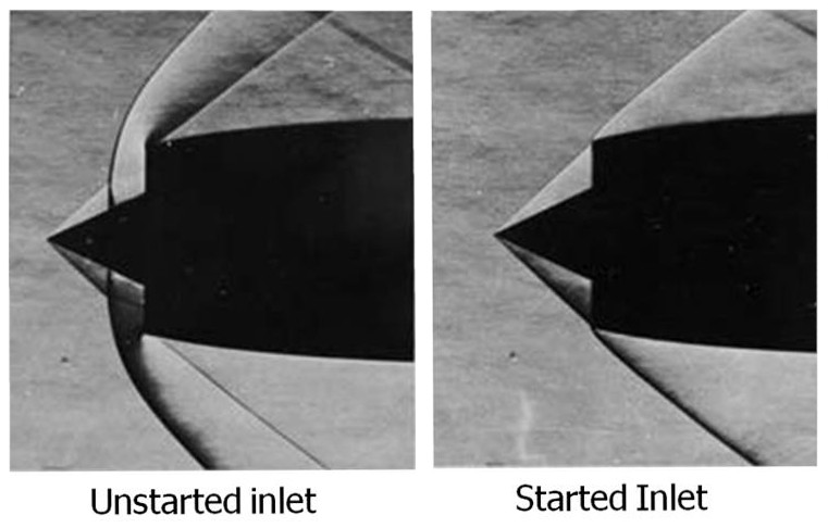
The lines in the image are shock waves. On a simple object like a wedge, the shock angle, wedge angle, and upstream and downstream Mach numbers (Mach number decreases through a shock) are all mathematically tied together. These relations are usually covered in a sophomore or junior level aerodynamics class.
The relation is most concisely summarized in NACA Report 1135. We will adopt its terminology for simplicity. Most importantly, Mach number is $\mathrm{M}$, the wedge angle (also called half angle) is $\delta$, and the shock angle is $\theta$. Let's do a quick example to reinforce these terms.
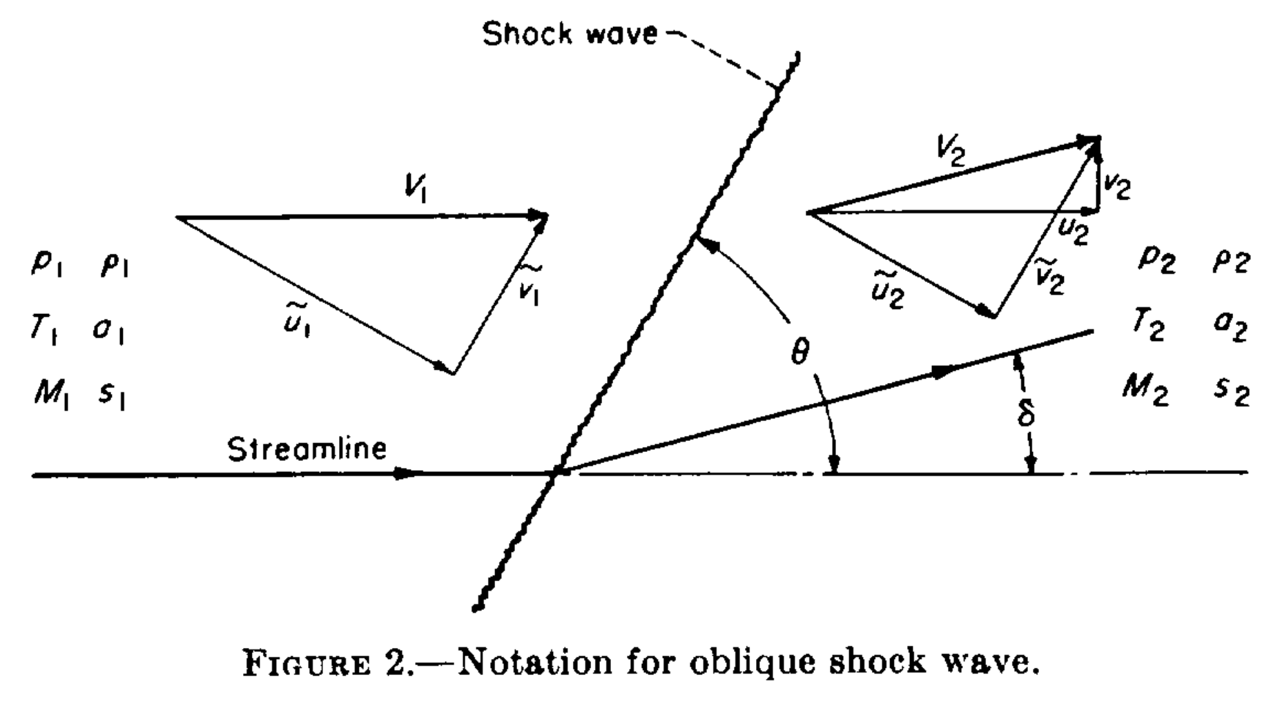
Warm-up Exercise
Given a wedge half-angle $\delta=10^{\circ}$ and shock angle $\theta=30^{\circ}$, calculate upstream Mach number.
Warm-up Solution
Using Equation 148b on page 622 of the Report, we have
\begin{eqnarray*} \mathrm{M}_1 &=& \sqrt{ \displaystyle\frac{2(\cot{\theta}+\tan{\delta})}{\sin{2\theta}-\tan{\delta}(\gamma + \cos{2\theta})} } \\ &=& \sqrt{ \displaystyle\frac{2(\cot{30^{\circ}}+\tan{10^{\circ}})}{\sin{60^{\circ}}-\tan{10^{\circ}}(1.4 + \cos{60^{\circ}})} } \\ &=& 2.681 \end{eqnarray*}This was easy enough, but of course real life is a little more challenging.
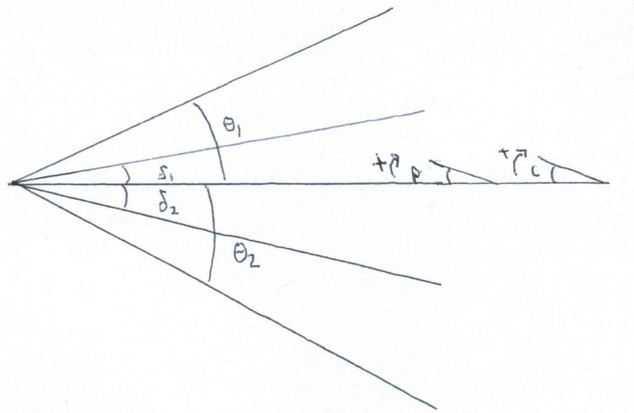
NOTE: from here on out, we are abandoning the subscripts $1$ and $2$ for upstream and downstream, they will now refer to the top and bottom edges of a wedge.
Problem
Using upper and lower shock angles and half angles, $\theta_1$, $\delta_1$, $\theta_2$, and $\delta_2$, calculate upstream Mach number. The subscripts $1$ and $2$ refer to the angle measured on the upper and lower wedge. You cannot assume a non-zero pitch $p$ or camera deflection angle $c$, and neither are known quantities (neglect flow angularity in the tunnel).
Down the Wrong Rabbit Hole
You may be first tempted to average the two deflection angles to get the half angle of the wedge. While this is simple and arguably accurate, it is not particularly helpful. There is an offset angle between them that can be caused by two (or more?) things: camera offset angle and the pitch angle of the wedge, $c$ and $p$.
Here's the problem with camera angle and pitch contributions to oblique shocks: changing the camera angle doesn't affect the physics of the shocks, but changing the pitch of the wedge does. Changing $p$ affects the effective half angle for the upper and lower wedges, thus influencing $\theta_1$ and $\theta_2$, but changing $c$ only offsets them. We need an approach that properly incorporates $c$ and $p$.
Solution
It out turns pitch angle is a sort of red herring; the solution lies in ignoring it (explicitly). Pitch is implicitly built into the relationship between the wedge angles. That's not to say it doesn't matter, averaging the wedge angles $\delta_1$ and $\delta_2$, for example, removes the implicit pitch contribution. As long as you don't mess with the half angles, pitch is accounted for.
If it helps, think of the top and bottom as separate wedges. Then we can apply equation 148b with camera angle. By using two equations, one each for top and bottom, we implicitly account for it.
$$\mathrm{M}_{1}^2 = \displaystyle\frac{2[\cot{(\theta_1+c)}+\tan{(\delta_1+c)}]} {\sin{(2\theta_1+2c)}-\tan{(\delta_1+c)}[\gamma + \cos{(2\theta_1+2c)}]} $$ And $$ \mathrm{M}_{2}^2 = \displaystyle\frac{2[\cot{(\theta_2-c)}+\tan{(\delta_2-c)}]} {\sin{(2\theta_2-2c)}-\tan{(\delta_2-c)}[\gamma + \cos{(2\theta_2-2c)}]} $$Subtract the two equations from each other (because $M_{1}=M_{2}$) and we are left with a single equation with the single unknown $c$ (remember, $\delta_1$, $\delta_2$, $\theta_1$ and $\theta_2$ will each be measured).
This is no picnic to solve analytically, but it can be easily tackled with Newton’s method. Newton requires the function and its derivative, which can be calculated using diff in MATLAB or sympy in Python (DON'T DIY). The MATLAB is
function [c,M] = find_offset(t1,t2,d1,d2)
%// returns offset (c) and Mach number

y=1.4;              %// Specific heat ratio
tol=1e-10;          %// Difference required to break loop
maxiterations=1000;
c=0;                %// Initial guess for offset csilon

for i=1:maxiterations
%// 1 corresponds to top edge, 2 corresponds to bottom edge

    M1=2*(cot(t1+c)+tan(d1+c))/(sin(2*(t1+c))-tan(d1+c)*(y+cos(2*(t1+c))));
    M2=2*(cot(t2-c)+tan(d2-c))/(sin(2*(t2-c))-tan(d2-c)*(y+cos(2*(t2-c))));

    dM1=-(2*cot(c+t1)^2-2*tan(c+d1)^2)/...
      (sin(2*c+2*t1)-tan(c+d1)*(cos(2*c+2*t1)+7/5)) ...
      -((2*cot(c+t1)+2*tan(c+d1))*(2*cos(2*c+2*t1)+...
      2*sin(2*c+2*t1)*tan(c+d1)-(tan(c+d1)^2+1)*(cos(2*c+2*t1)+7/5)))...
      /(sin(2*c+2*t1)-tan(c+d1)*(cos(2*c+2*t1)+7/5))^2;

    dM2=(2*cot(t2-c)^2-2*tan(d2-c)^2)...
      /(sin(2*t2-2*c)-tan(d2-c)*(cos(2*t2-2*c)+7/5))+...
      ((2*cot(t2-c)+2*tan(d2-c))*(2*cos(2*t2-2*c)+...
      2*sin(2*t2-2*c)*tan(d2-c)-(cos(2*t2-2*c)+7/5)*(tan(d2-c)^2+1)))...
      /(sin(2*t2-2*c)-tan(d2-c)*(cos(2*t2-2*c)+7/5))^2;

    %// Newtons Method
    Mdiff=M1-M2;
    dMdiff=dM1-dM2;
    diff=Mdiff/dMdiff;
    c=c-diff;

    %// Check for early break
    if abs(diff) < tol
      break
    end

end %// for loop
end %// function
If you're a skeptic, the alarm bells might be ringing. You can't just ignore what components factor into the offset angle...can you?
This is hard to prove (frankly I'm not sure how one would rigorously), and even a rigorous mathematical proof is probably not very exciting The below test cases make a good case for the algorithm's veracity. Here $\delta$ is the "original" half angle of the wedge; it is not used except to help generate test cases.
| $\mathrm{M}$ | $\delta$ | $p$ | $c$ | $\delta_1=(\delta+p)-c$ | $\delta_2=(\delta-p)+c$ | $\theta_1=\theta(\mathrm{M},\delta+p)-c$ | $\theta_2=\theta(\mathrm{M},\delta-p)+c$ |
|---|---|---|---|---|---|---|---|
| $2$ | $10^{\circ}$ | $0^{\circ}$ | $0^{\circ}$ | $10^{\circ}$ | $10^{\circ}$ | $\theta_{10}-0^{\circ}=39.31^{\circ}$ | $\theta_{10}+0^{\circ}=39.31^{\circ}$ |
| $2$ | $10^{\circ}$ | $5^{\circ}$ | $5^{\circ}$ | $10^{\circ}$ | $10^{\circ}$ | $\theta_{15}-5^{\circ}=40.34^{\circ}$ | $\theta_{5}+5^{\circ}=39.30^{\circ}$ |
| $2$ | $10^{\circ}$ | $5^{\circ}$ | $0^{\circ}$ | $15^{\circ}$ | $5^{\circ}$ | $\theta_{15}-0^{\circ}=45.34^{\circ}$ | $\theta_{5}+0^{\circ}=34.30^{\circ}$ |
| $2$ | $10^{\circ}$ | $0^{\circ}$ | $5^{\circ}$ | $5^{\circ}$ | $15^{\circ}$ | $\theta_{10}-5^{\circ}=34.31^{\circ}$ | $\theta_{10}+5^{\circ}=44.31^{\circ}$ |
| $2$ | $10^{\circ}$ | $5^{\circ}$ | $-5^{\circ}$ | $20^{\circ}$ | $0^{\circ}$ | $\theta_{15}+5^{\circ}=50.34^{\circ}$ | $\theta_{5}-5^{\circ}=29.30^{\circ}$ |
| $2$ | $10^{\circ}$ | $-5^{\circ}$ | $5^{\circ}$ | $0^{\circ}$ | $20^{\circ}$ | $\theta_{5}-5^{\circ}=29.30^{\circ}$ | $\theta_{15}+5^{\circ}=50.34^{\circ}$ |
| $2$ | $15^{\circ}$ | $-5^{\circ}$ | $5^{\circ}$ | $5^{\circ}$ | $25^{\circ}$ | $\theta_{10}-5^{\circ}=34.31^{\circ}$ | $\theta_{20}+5^{\circ}=58.42^{\circ}$ |
Here, $\theta(\mathrm{M},\delta)$ denotes a function to calculate shock angle from Mach number and wedge angle. This can be accomplished with equation 150a (the solution of which was the motivation for the previous post). The four test shock angle values are $\theta_{5}=34.30^{\circ}$, $\theta_{10}=39.31^{\circ}$, $\theta_{15}=45.34^{\circ}$, $\theta_{20}=53.42^{\circ}$.
If you write your own tests, stay away from negative and non-physical angles. Furthermore, negative angles are properly handled with Prandtl-Meyer expansion, which uses a different set of assumptions and equations.
I ran them through the code (I encourage you to do the same) and they all spit out the same Mach number, despite having either the same offset angle from different sources, or different offset angles.
If you want to run the code yourself, you can download it here. NOTE: the angles in this code are all in degrees (contrary to the snippet above).
Other Considerations
Earlier we neglected tunnel angularity. This was essential to keep our problem constrained. Solving for (one component) tunnel angularity can be achieved if we know the camera offset angle or pitch angle, but not if we know neither (and no other information). It is not a perfect substitution, but it is a simple enough exercise (and will of course be left to the reader). Depending on your setup, you may trust you camera angle more than your tunnel angularity.
Speeding up Code with Vectorization
Posted on January 15, 2016
In a previous post we numerically solved the heat equation with an explicit finite difference formulation, one of the simpler 2D problems in numerical analysis.
In this post we are going to speed up that computation with some vectorization. Results show we can more than double the speed of our code with some simple changes (but also that we can make it dangerously slow if implemented incorrectly).
The code examples below are in MATLAB, but you can take advantage of vectorization with other interpreted languages such as Python as well. You can read more about vectorization of MATLAB code here.
Step 1: Initialize VariablesNot much changes in this section except that we will replace nx and ny with np and use a square mesh for simplicity.
%Initialize Variables
dt=.005;                 %time step
nts=500;                 %number of time steps
alpha=.01;               %thermal diffusivity
l=1;                     %reference length plate
np=50;                   %number of points (x and y)
dx=l/(np-1); dy=dx;      %discretized distance

%Temperature and derivatives stored in 2D arrays
u = zeros(np); uxx = zeros(np); uyy = zeros(np);
Step 2: Apply Boundary Conditions
In the following sections we will use snippets outlined in yellow to show the original code, green to show standard vectorization, and red to show sliced vectorization. In the original code (below) we looped through the two edges to apply the boundary conditions
%Boundary Conditions, original loop
for i=1:np
   u(1,i)=1;
end

for i=1:np
   u(i,np)=1;
end
This is a one-time computation so there isn’t significant time saved by changing this, but regardless we can do better by both simplifying and speeding up our code.
%Boundary Conditions, % Vectorization without slicing
u(1,:)=u(1,:)+1;
u(:,np)=u(:,np)+1;
u(1,np)=1;
We had to correct the value of at the coordinate $(1,np)$ because are adding to it twice. So why didn’t we just take a slice of the array, like 2:np? Here is what it looks like with sliced vectorization
%Boundary Conditions, vectorization with slicing
part=2:np;
u(1,:)=u(1,:)+1;
u(part,np)=u(part,np)+1;
This looks a little nicer, but actually has a significant impact on run time. Results of a benchmark comparison with 10,000,000 test cases is shown in the table below
| Original loop | 13.46 s |
| Vectorization with slicing | 33.29 s |
| Vectorization without slicing | 10.29 s |
So while sliced vectorization looks nice and doesn't require a correction, it more than triples execution time.
Step 3: Time LoopThe more important changes come with the code inside of the time loop, so let's shift our focus there. Here is the original code.
% Original Loop
for t=1:nts

   %Calc the Spatial 2nd Derivative, Centered in Space
   for i=2:np-1
      for j=2:np-1
         uxx(i,j)=(u(i+1,j)-2*u(i,j)+u(i-1,j))/(dx)^2;
         uyy(i,j)=(u(i,j+1)-2*u(i,j)+u(i,j-1))/(dy)^2;
      end
   end

   %Update Temperature, Forwards in Time
   for i=2:np-1
      for j=2:np-1
         u(i,j)=u(i,j)+alpha*(uxx(i,j)+uyy(i,j))*dt;
      end
   end
end
We can simplify this code greatly with vectorization. The code below requires corrections, but improves run time drastically.
% Vectorization without slicing
for t=1:nts

   %Calc the Spatial 2nd Derivative, Centered in Space
    for i=2:np-1
        uxx(i,:)=(u(i+1,:)-2*u(i,:)+u(i-1,:))/(dx)^2;
        uyy(:,i)=(u(:,i+1)-2*u(:,i)+u(:,i-1))/(dy)^2;
    end
    uxx(2,1)=0; %correction
    uyy(np,np-1)=0; %correction
    % Note, we do not need to correct other BC points since the uxx,uyy=0 - it would be safer to tho

    %Update Temperature, Forwards in Time
    u=u+alpha*(uxx+uyy)*dt;
end
Note that we had to once again make a correction after the vectorized calculations. Here is what it looks like with sliced vectorization that wouldn't require corrections
% Vectorization with slicing
part=2:np-1;
for t=1:nts

    %Calc the Spatial 2nd Derivative, Centered in Space
    for i=2:np-1
        uxx(i,part)=(u(i+1,part)-2*u(i,part)+u(i-1,part))/(dx)^2;
        uyy(part,i)=(u(part,i+1)-2*u(part,i)+u(part,i-1))/(dy)^2;
    end

    %Update Temperature, Forwards in Time
    u=u+alpha*(uxx+uyy)*dt;
end
Once again this looks much nicer but as we see below, the slices are once again much slower.
The comparison of all three methods run 30 times with 5000 time steps each are shown in the following table.
| Original loop | 25.48 s |
| Vectorization with slicing | 84.31 s |
| Vectorization without slicing | 10.68 s |
With properly implemented vectorization we can drastically speed up our code, but as the results show it must be done carefully and tested to ensure both accuracy (by making the proper corrections) and speed.
Projectile Motion with (Quadratic) Drag
Posted on October 31, 2013
Projectile motion is discussed and worked out in nearly every college physics, calculus, and dynamics class, but examples always seem to neglect or over-simplify drag. In this post we will tackle an analytic solution that models drag for a falling object.
Let’s suppose we are dropping a ball from a height \(h_0\) with a velocity \(v_0\). In a vaccuum, the only force is gravity, $mg$. Then projectile motion without drag begins with Newton’s second law $$F_{net}=mg=ma \rightarrow a=g.$$ Acceleration can then be twice integrated with respect to time, yielding $$p(t)=\frac{g}{2}t^2+v_0t+h_0.$$ Given a constant force (i.e. not dependent on time or velocity) this is a simple integration with respect to time and the math is rather elementary. We can make it much more challenging by inserting an additional force term, drag, which is dependent on velocity: $$F=mg-D =ma \rightarrow a=g-D/m.$$ Many approximations for drag can be applied, but the most accurate model is $$D=1/2 \rho v^2\cdot c_d\cdot A.$$ Here \(c_d\) is coefficient of drag (dimensionless), A is the cross-sectional area, and \(\rho\) is the density of the medium the object is falling (e.g. air is $1.225 ~ \mathrm{kg}/\mathrm{m}^3$). Let’s jump into the math. $$a=g-D/m=g-\frac{\rho\cdot c_d\cdot A}{2m}v^2.$$ Now let \(a=dv/dt\) and for simplicity let \(k^2=\frac{\rho\cdot c_d\cdot A}{2mg}\). Coincidentally, $\frac{1}{k}$ is also the terminal velocity of a falling object. We have \begin{eqnarray} \frac{dv}{dt} &=& g-gk^2 v^2 \\ g\cdot dt &=& \frac{dv}{1-k^2 v^2}. \end{eqnarray} In its current form, this is not a simple integration. It can be evaluated with the hyperbolic arc-tangent, but to keep the equations in terms of more recognizable functions we will instead apply a partial fraction expansion $$\frac{dv}{1-k^2 v^2}=\frac{1}{2k}\left[\frac{dv}{v-1/k}-\frac{dv}{v+1/k}\right].$$
If this is confusing, you can review partial fraction expansions here
Now we can integrate \begin{eqnarray} g\cdot dt &=& \frac{1}{2k} \left[\frac{dv}{v+1/k}-\frac{dv}{v-1/k}\right]. \\ g\cdot t &=& \frac{1}{2k} \left[\ln(v+1/k)-\ln(v-1/k)\right]+C_1. \end{eqnarray}
We now have time as a function of velocity, but that isn’t very useful. Let’s see if we can solve for $v$: \begin{eqnarray} g\cdot t &=& \frac{1}{2k} \left[ \ln(v+1/k)-\ln(v-1/k) \right] +C_1 \\ g\cdot t &=& \frac{1}{2k}\cdot\ln\left[\frac{v+1/k}{v-1/k}\right]+C_1 \\ 2gk\cdot t+C_2 &=& \ln\left[\frac{v+1/k}{v-1/k}\right]\\ \end{eqnarray}
Now we can exponentiate both sides
\begin{eqnarray} Ce^{2gk\cdot t}=\frac{v+1/k}{v-1/k}=\frac{2/k}{v-1/k}+1. \\ \end{eqnarray} Now we can solve for $v$. \begin{eqnarray} v &=& \frac{2/k}{Ce^{2gk\cdot t}-1}+1/k. \\ &=& \frac{1}{k}\left(\frac{2}{Ce^{2gk\cdot t}-1}+1\right). \\ \end{eqnarray} Now we eliminate that pesky \(C\) by applying an initial condition for velocity. We are simply dropping something so let \(v(0)=0\).
We have \begin{eqnarray} v &=& \frac{1}{k}\left(\frac{2}{Ce^{2gk\cdot 0}-1}+1 \right) \\ &=& \frac{1}{k}\left(\frac{2}{C-1}+1 \right) \rightarrow C=-1. \end{eqnarray} Therefore $$v = \frac{1}{k}\left(1-\frac{2}{e^{2gk\cdot t}+1}\right).$$ Velocity is all fine and dandy, but what we are really after is position. This requires one more integration, but fortunately it’s a little simpler: This takes a little rewriting u-substitution. We have \begin{eqnarray} \frac{dp}{dt} &=& \frac{1}{k}\left(1-\frac{2}{e^{2gk\cdot t}+1}\right) \\ &=& \frac{1}{k}\left(1-\frac{2e^{2gk\cdot t}+2}{e^{2gk\cdot t}+1}+\frac{2e^{2gk\cdot t}}{e^{2gk\cdot t}+1}\right) \\ &=& \frac{1}{k}\left(1-2+\frac{2e^{2gk\cdot t}}{e^{2gk\cdot t}+1}\right). \end{eqnarray}
Now this is in a form where we can intuitively apply $u$-substitution. We have \begin{eqnarray} p=\frac{1}{gk^2}\ln[e^{2gk\cdot t}+1]-\frac{t}{k}+C. \end{eqnarray} Now if we apply the initial condition \(h(0)=h_0\) we have \begin{eqnarray} p &=& \frac{1}{gk^2} \ln\left[e^{2gk\cdot t}+1\right]-\frac{\ln(2)}{gk^2}-\frac{t}{k}+h_0. \\ &=& \frac{1}{gk^2} \ln\left[\frac{e^{2gk\cdot t}+1}{2}\right]-\frac{t}{k}+h_0. \end{eqnarray}
Let's put this to use with a quick example. Let's say we are dropping two balls off a tower $56~\mathrm{m}$ tower. They have the same cross-sectional area $A=1/3 ~ \mathrm{m}^2$ and drag coefficient $c_d=0.5$, but have different masses of $1 ~ \mathrm{kg}$ and $5 ~ \mathrm{kg}$. We can use the above formula to find how long it takes them to hit the ground.
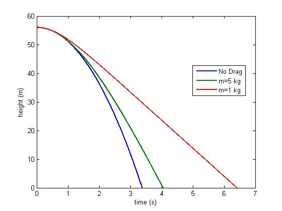
Clearly accounting for drag is important if the object falling is very light, very large, or is falling through a medium with a high density.