Newton’s Method for Polynomials

---

Posted on April 14, 2018

---

Newton’s Methods is a useful tool for finding the roots of real-valued, differentiable functions. A drawback of the method is its dependence on the initial guess. For example, all roots of a 10th degree polynomial could be found with 10 very good guess. However, 10 very bad guesses could all point to the same root.

In this post, we will present an iterative approach that will produce all roots. Formally

Newton's method can be used recursively, with inflection points as appropriate initial guesses, to produce all roots of a polynomial.

Motivation

While working through the Aero Toolbox app, I needed to solve a particular cubic equation (equation 150 from NACA Report 1135, if you're interested).

I needed to find all 3 roots. The cubic equation is well known, but long and tedious to code up. I had already been implementing Newton’s Method elsewhere  in the app and wanted to use that. The challenge though, as is always the challenge with using Newton’s Method on functions with multiple roots is robustly finding all of them.

This particular cubic was guaranteed to have three distinct roots. The highest and lowest were easy; I was solving for the square of the sine of particular angles so $0$ and $1$ are good starting points. The middle root was not so easy. After some brainstorming, I took a stab at a possible guess: the inflection point. Low and behold, it (without fail) always converged the middle root.

Delving Further

So why did the inflection point always converge to the middle root?  Let's explore!

We'll start with a simple example: a polynomial with unique, real roots.  The root is either identical to the inflection point, to the left of it, or to the right of it.

Assume WLOG that the derivative is positive in this region.  There will always be a root in between the inflection point and the local min/max to each side (This statement requires proof, which will of course be left to the reader ;) ).  Let's examine all three cases.

Case 1: Inflection Point is a root

You are at a root, so Newton's Method is converged.  Both the function $p$ and its derivative $p'$ are $0$, so as long as your implementation avoids division by zero or erratic behavior close to $\frac{0}{0}$, you're in the clear.

Case 2: Root to the left of the inflection point

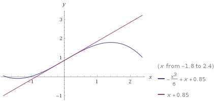
The slope will flatten out to the left of the inflection point, therefore the tangent line will intersect the $x$-axis before $p$ does.  That means Newton's Method will not overshoot the root. In subsequent guesses, this same pattern will hold.

Consider an example in the graph below, $p(x)=-\frac{x^3}{6}+x+0.85$, shown in blue.  In the graph below, the tangent line is shown in purple.  The intersection of the tangent line and the $x$-axis is the updated guess.

Case 3: Root to the right of the inflection point

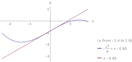
The logic is the same, but with signs reversed.  The root is to the right of the inflection point.  All guesses will move right monotonically without overshooting the root.

Consider an example in the graph below of a different polynomial, $p(x)=-\frac{x^3}{6}+x-0.85$, shown in blue.  In the graph below, the tangent line is shown in purple.  The intersection of the tangent line and the $x$-axis is the updated guess.

Generalizing to Higher Order Polynomials

This method can be generalized to higher orders in a recursive fashion. For an $n$th order polynomial $p$ we can use the roots 2nd derivative $p’’$ (degree $n-2$) as starting guesses for the roots of $p$. To find the roots of $p’’$, you need the roots of $p’’’’$ and so on. Also, as part of the method, you need $p’$. Therefore, all derivatives of the polynomial are required.

Two functions are required.  First,  a simple implementation of Newton's method

def newton_method(f, df, g, deg):
    max_iterations = 100
    tol = 1e-14
    for i in xrange(max_iterations):
        fg = sum([g ** (deg - n) * f[n] for n in xrange(len(f))])
        dfg = float(sum([g ** (deg - n - 1) * df[n] for n in xrange(len(df))]))
        if abs(dfg) < 1e-200:
            break
        diff = fg / dfg
        g -= diff
        if abs(diff) < tol:
            break
    return g
        

The second part is iteration

def roots_newton(coeff_in):
    ndof = len(coeff_in)
    deg = ndof - 1
    coeffs = {}
    roots = [([0] * row) for row in xrange(ndof)]

    # Make coefficients for all derivatives
    coeffs[deg] = coeff_in
    for i in xrange(deg - 1, 0, -1):
        coeffs[i] = [0] * (i+1)
        for j in range(i+1):
            coeffs[i][j] = coeffs[i + 1][j] * (i - j + 1)

    # Loop through even derivatives
    for i2 in xrange(ndof % 2 + 1, ndof, 2):
        if i2 == 1:   # Base case for odd polynomials
            roots[i2][0] = -coeffs[1][1] / coeffs[1][0]
        elif i2 == 2: # Base case for even polynomials
            a, b, c = coeffs[2]
            disc = math.sqrt(b ** 2 - 4 * a * c)
            roots[2] = [(-b - disc) / (2 * a), (-b + disc) / (2 * a)]
        else:
            guesses = [-1000.] + roots[i2 - 2] + [1000.] #Initial guesses of +-1000
            f = coeffs[i2]
            df = coeffs[i2 - 1]
            for i, g in enumerate(guesses):
                roots[i2][i] = newton_method(f, df, g, i2)
    return roots[-1]

This method will also work for polynomials with repeated roots.  However, there is no mechanism for finding complex roots.

Comparison to Built-in Methods

The code for running these comparisons is below.

 #repeated roots
ps = [[1, 2, 1], 
[1, 4, 6, 4, 1], 
[1, 6, 15, 20, 15, 6, 1], 
[1, 8, 28, 56, 70, 56, 28, 8, 1],
[1, 16, 120, 560, 1820, 4368, 8008, 11440, 12870, 11440, 8008, 4368, 1820, 560, 120, 16, 1],

#unique roots from difference of squares
[1, 0, -1], 
[1, 0, -5, 0, 4], 
[1, 0, -14, 0, 49, 0, -36], 
[1, 0, -30, 0, 273, 0, -820, 0, 576],
[1, 0, -204, 0, 16422, 0, -669188, 0, 14739153, 0, -173721912, 0, 1017067024, 0, -2483133696, 0, 1625702400]
]
n = 1000
for p in ps:
avg_newton = time_newton(p, n)
avg_np = time_np(p, n)
print len(p)-1, avg_newton, avg_np, avg_newton/avg_np

The comparison to built-in methods is rather laughable.  A comparison to the numpy.roots subroutine is showed below.  Many of the numpy routines are optimized/vectorized etc. so it isn't quite a fair comparison.  Still, the implementation of Newton's Method shown here appears to have $O(n^3)$ runtime for unique roots (and higher for repeated roots), so it's not exactly a runaway success.

Two tables,  below, summarize root-finding times for  two polynomials.  The first is for repeated roots $(x+1)^n$.  The second is for unique roots, e.g. $x^2-1$, $(x^2-1)\cdot(x^2-4)$, etc.

$n$	Newton	np.roots	times faster
2	$6.10\times 10^{-6}$	$1.41\times 10^{-4}$	$0.0432$
4	$5.36\times 10^{-4}$	$1.15\times 10^{-4}$	$4.68$
6	$2.50\times 10^{-3}$	$1.11\times 10^{-4}$	$22.5$
8	$5.54\times 10^{-3}$	$1.23\times 10^{-4}$	$44.9$
16	$9.66\times 10^{-2}$	$1.77\times 10^{-4}$	$545.9$

$n$	Newton	np.roots	times faster
2	$5.57\times 10^{-6}$	$1.03\times 10^{-4}$	$0.0540$
4	$2.71\times 10^{-4}$	$1.04\times 10^{-4}$	$2.60$
6	$7.43\times 10^{-4}$	$1.09\times 10^{-4}$	$6.82$
8	$1.43\times 10^{-3}$	$1.21\times 10^{-4}$	$11.8$
16	$1.26\times 10^{-2}$	$1.72\times 10^{-4}$	$73.1$