Finite Difference Solution of the Heat Equation on a Structured Mesh
Posted on November 19, 2013
Introduction
In this post we will numerically solve the heat equation with an explicit finite difference formulation.
Objective: Obtain a numerical solution for the 2D Heat Equation in MATLAB using an explicit finite difference formulation.
Helpful background: basic understanding of PDEs (partial differential equations), basic MATLAB coding (for loops and arrays), and basic derivative approximations with finite differences.
Modeling the problem
First let’s introduce the heat equation. The heat equation in two dimensions is $$u_t=\alpha(u_{xx}+u_{yy})$$ where $u(x,y,t)$ is a function describing temperature and $\alpha$ is thermal diffusivity.
Numerically discretizing the equations We are going to solve the heat equation numerically. There are many methods that solve this, but the simplest is an explicit finite difference formulation. Explicit means the solution at a certain time step depends only on previous step, as opposed to implicit (see here) where the solution depends on next time step. Finite differences are a simple way to use neighboring grid points to approximate derivatives.
We will use the central difference approximation for our second derivatives. The approximations for $u_{xx}$ and $u_{yy}$ are \begin{eqnarray} u_{xx}(i,j)&=&\displaystyle\frac{u(i+1,j)-2\cdot u(i,j)+u(i-1,j)}{(\Delta x)^2} \\ u_{yy}(i,j)&=&\displaystyle\frac{u(i,j+1)-2\cdot u(i,j)+u(i,j-1)}{(\Delta y)^2}. \end{eqnarray} These are all at time $n$ (they are not exponents). We will use the forward difference approximation for $u_t$. We have
$$ u_t^n=\frac{u^{n+1}-u^n}{\Delta t}.$$
This is for every point $(i,j)$. Now we can take these 3 expressions, combine them, and solve for $u^{n+1}$.
\begin{eqnarray} u_t^n(i,j) &=& \alpha(u_{xx}^n(i,j)+u_{yy}^n(i,j)) \\ \frac{u^{n+1}(i,j)-u^n(i,j)}{\Delta t} &=& \alpha\left[\frac{u(i+1,j)-2\cdot u(i,j)+u(i-1,j)}{(\Delta x)^2}+ \frac{u(i,j+1)-2\cdot u(i,j)+u(i,j-1)}{(\Delta y)^2}\right] \\ u^{n+1}(i,j) &=& u^n(i,j)+\alpha\cdot dt\left[ \frac{u(i+1,j)-2\cdot u(i,j)+u(i-1,j)}{(\Delta x)^2}+\frac{(u(i,j+1)-2\cdot u(i,j)+u(i,j-1)}{(\Delta y)^2}\right] \end{eqnarray}
A quick look at stability The formulation we used (forward in time, centered in space) is only conditionally stable. We can show (but won’t here) with Von Neumann Stability Analysis, that we need the discretized time step $\Delta t$ to satisfy $$ \Delta t< \frac{\Delta x^2}{4\alpha}.$$Once you have your code written it is easy to empirically test this.
The code
Let’s set up a specific example. A $1x1$ flat plate has a thermal diffusivity of $\alpha=.01$. The temperature is fixed at $u=1$ on the top and right edges and $u=0$ on the bottom and left edges. Elsewhere, the initial temperature is $u=0$. Find the temperature distribution over time.
(Note: I left off any units and have some simplified numbers for temperature and plate dimensions. Feel free to change them as you please, but make sure your formulation is still stable.)
Now let’s lay out the code. We are going to break it up into three steps: Initialize relevant physical values, set the boundary conditions, and set up the time loop. The time loop will consist of calculating the derivatives at each point, updating the temperature for each point, and then updating the visualization.
Step 1: Initialize variables We will start by initializing relevant physics variables for the time step size, number of time steps, thermal diffusivity, reference plate length, number of points in the x and y direction, and the spatial discretization $\Delta x$ and $\Delta y$.
You can also preallocate the matrices for $u$, $u_{xx}$, and $u_{yy}$.
%Initialize Variables
dt=.005;                   %time step
nts=500;                   %number of time steps
alpha=.01;                 %thermal diffusivity
l=1;                       %reference length plate
nx=50; ny=50;              %number of points in the x and y directions
dx=l/(nx-1); dy=l/(ny-1);  %discretized distance in between points

%Temperature and the derivatives will be stored in a two dimensional array
u = zeros(nx,ny); uxx = zeros(nx,ny); uyy = zeros(nx,ny);
Step 2: Apply Initial and Boundary Conditions
%Initial/Boundary Conditions
for i=1:ny
   u(1,i)=1;
end

for i=1:nx-1
   u(i,ny)=1;
end
Step 3: Time Loop Here is the meat of the code. The time loops has three components, first calculate the second derivatives, then update temperature, then update the visualization.
for t=1:nts
   %Calc the Spatial 2nd Derivative, Centered in Space
   for i=2:nx-1
      for j=2:ny-1
         uxx(i,j)=(u(i+1,j)-2*u(i,j)+u(i-1,j))/(dx)^2;
         uyy(i,j)=(u(i,j+1)-2*u(i,j)+u(i,j-1))/(dy)^2;
      end
   end

   %Update Temperature, Forwards in Time
   for i=2:nx-1
      for j=2:ny-1
         u(i,j)=u(i,j)+alpha*(uxx(i,j)+uyy(i,j))*dt;
      end
   end

   %Visualization
   contourf(u)
   axis equal
   M(t) = getframe;
end %time loop
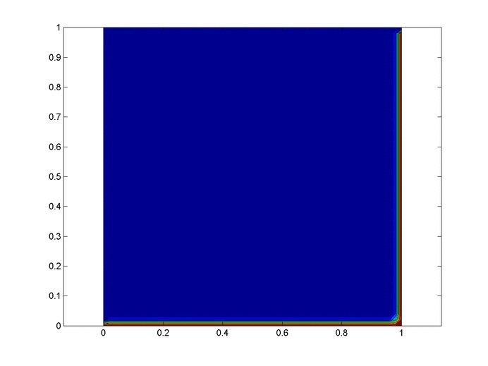
Results
Below are 2 GIFs (one is a contour plot, the other is a surface plot) of the temperature distribution over time.