Implicit finite difference formulation on an unstructured mesh

Posted on March 17, 2014

Introduction

Objective: Obtain a numerical solution for the 2D Heat Equation using an implicit finite difference formulation on an unstructured mesh in MATLAB. The temperature distribution over time for an example problem described below will look something like this:

Helpful background: basic understanding of PDEs (partial differential equations), basic MATLAB coding (for loops, arrays and structure arrays), and solution methods for matrix equations.

Modeling the physics

First let’s introduce the heat equation. The heat equation in two dimensions is $$u_t=\alpha(u_{xx}+u_{yy})$$ where $u(x,y,t)$ is a function describing temperature and $\alpha$ is thermal diffusivity.

Numerically discretizing the equations We are going to solve the heat equation numerically with finite differences on an unstructured mesh. This is a fairly non-standard approach; when numerical analysts encounter difficult geometries they typically move on from cartesian finite difference for coordinate transformations, or other methods like finite volumes or finite elements on unstructured meshes.

We will keep as close as possible to the true nature of finite difference without using coordinate transformations. Our previous post did this as well, but what makes this method more desirable is the flexibility that comes from unstructured meshing. With an unstructured mesh, it is easier to mesh around complex geometries and add local refinement.

Approximating derivatives To create discretized equations we will need approximations for the second derivatives $u_{xx}$ and $u_{yy}$. We will go back to a Taylor series expansion, but this time extend it in in two dimensions. Consider a function $u$ at points $u_0=u(x_0,y_0)$ and $u_1=u(x_1,y_1)$ with $x_1=x_0+\Delta x$ and $y_1=y_0+\Delta y$. Then the two dimensional Taylor series expansion is $$ u_1 \approx u_0 + u_x\Delta x +u_y\Delta y +u_{xx}\Delta x^2 +u_{yy}\Delta y^2 +u_{xy}\Delta x \Delta y $$ We will treat $\Delta x$, $\Delta y$, $\Delta x^2$, $\Delta y^2$, $\Delta x\Delta y$, as coefficients and let the derivatives be the unknowns. Then we have a linear equation with five unknowns, $u_x$, $u_y$, $u_{xx}$, $u_{yy}$, and $u_{xy}$. That means to solve for all first and second derivatives requires five linearly independent equations, which we can get if we have $n \geq 5$ neighboring points that aren't collinear in the same direction.

Set it up as $A\textbf{x}=\textbf{b}$ where \[ \textbf{b} = \left[ \begin{array}{c} u_1-u_0 \\ u_2-u_0 \\ … \\ u_n-u_0 \end{array} \right] \] \[ \textbf{x} = \left[ \begin{array}{c} u_x \\ u_y \\ u_{xx} \\ u_{yy} \\ u_{xy} \\ \end{array} \right] \]

and $A$ is the coefficient matrix.

As one might guess, this results in approximations with second order accuracy for the first derivatives but only first order accuracy for the second derivatives, which is not acceptable accuracy. There are different ways to address this but the simplest is to add the third derivative terms to our equations. There are four third derivatives $u_{xxx}$, $u_{yyy}$, $u_{xxy}$, and $u_{xyy}$. This means we will need to use information from nine neighboring points to attain second order accuracy.

Now you may be wondering, how will we pick the nine neighboring points that best solve the physical problem? To best capture the physics we want equal weight from the surrounding points. However, unstructured meshes have a varying number of neighboring points, and often times have less than nine. To address this problem we will get greedy - we will not take just all neighboring points, but all the neighbors of neighboring points. This will leave us with much more than nine equations (generally 20-30) for only nine unknowns.

To best solve the overdetermined system we will use the least squares method. For an overdetermined system $A\textbf{x}=\textbf{b}$ the least squares solution is $$ \textbf{x}=\left[ (A^TA)^{-1}A^T \right] \textbf{b}$$ Let $\textbf{d}$ be the sum of the fourth and fifth rows of $(A^TA)^{-1}A^T$. Then we can write $$ (u_{xx}+u_{yy})_{x_0,y_0} = \textbf{d}\textbf{b}.$$ Since the mesh does not move we can use the same coefficients to calculate derivatives at every time step. Therefore these least squares calculations and assembly $\textbf{d}$ vectors (one for each node) of only need to be carried out once.

As we will show later in the code it is not good if the matrix has linearly dependent rows. To avoid this one could add an error check that eliminates $\Delta x$ and $\Delta y$ pairs that have close to the same angle. The closer points are to being linearly independent, the worse the condition of the matrix $A$. That said, if the angles differ by $180^{\circ}$ then rows are still linearly independent due to the nature of the coefficients.

Now that we have a way to calculate the derivatives, we can implement a formulation. We have shown the explicit FTCS formulation in two previous posts, so in this post we will just focus on an implicit method. We will use the Crank-Nicolson method (for more, check this paper on finite differences with the heat equation).

Implicit formulation (Crank-Nicolson)

The approximation becomes \begin{eqnarray} u_t^n &=& \alpha\cdot(u_{xx}+u_{yy}) \\ \frac{u^{n+1}-u^n}{dt} &=& \frac{\alpha}{2} \left[ (u_{xx}+u_{yy})^{n+1} + (u_{xx}+u_{yy})^n \right] \\ u^{n+1} - \frac{\alpha\cdot dt}{2}(u_{xx}+u_{yy})^{n+1} &=& u^n + \frac{\alpha\cdot dt}{2}(u_{xx}+u_{yy})^n \\ u^{n+1} - \frac{\alpha\cdot dt}{2} \textbf{d}\textbf{b}^{n+1} &=& u^n + \frac{\alpha\cdot dt}{2} \textbf{d}\textbf{b}^n \end{eqnarray} The left hand side of the equation is called the implicit side and contains the unknowns $u^{n+1}$ and $\textbf{b}^{n+1}$. The right hand side is all known values ($u^n$ and $\textbf{b}^n$ are from the previous time step) and is called the explicit side.

If we create an equation like this for each of the $n$ point in our domain then we have a system of $n$ equations with $n$ unknowns in the form $A\textbf{x}=\textbf{b}$ where $\textbf{x}$ is all of the $u^{n+1}$ values, $\textbf{b}$ is the explicit side, and $A$ is the coefficients from the left hand side.

Example problem

For example we will use the same physical problem as in part 2 (the only difference is the length scale). A $1x1$ flat plate has a thermal diffusivity of $\alpha=.001$. The temperature is fixed at $u=1$ on an inner circular boundary and is fixed at 0 on four outer boundaries. Elsewhere, the initial temperature is $u=0$. Find the temperature distribution over time.

Meshing

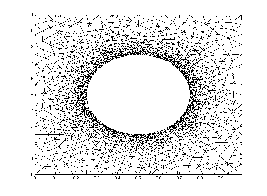
Much of the best meshing software is propietary and expensive, but there are some good free programs like Gmsh. We will implement code to read in and use a *.msh file.

We will test out the mesh below. It has $1,992$ nodes.

The code

Now let’s lay out the code. We are going to break it up into three steps: initialize relevant physical parameters, import the mesh, set the boundary conditions, assemble the coefficient matrix, and set up the time loop.

Step 1: Initialize physical parameters

%Physical Quantities
nts=100; ntsabout=100;
dt=.03; alpha=.001; c=alpha*dt/2;

Step 2: Import the Mesh

[xyz,mesh,nn,tri,bnd,map]=importmesh2('circle_fine.msh');

The function will return

xyz: the nodes in a (nn,2) where nn is the number of points in the mesh.
mesh: A structure array containing the fields nbr (neighboring points), dx and dy (the distances to respective points), coeff the coefficients of the derivative approximation, and bnd, the boundary type of the point.
tri: the “connectivity of the mesh (for visualizations).
nn: The number of nodes in the mesh
bnd: a list of the nodes in the boundary. Only necessary for an implicit formulation.
map: The points in the mesh not on a boundary.

I will not include the importmesh2 code in this post but you can access the text here.

Step 3: Apply Initial and Boundary Conditions

%Initialize arrays
T = zeros(nn,1); A=zeros(nn); b=zeros(nn,1);

%Initial conditions
for n=bnd
    if mesh(n).bnd==5
        T(n)=1;
    end
end

Step 4: Assemble coefficient matrix and boundary contribution to the rhs vector

for i=bnd
    A(i,i)=1;
end

for i=map
    A(i,i)=1+c*mesh(i).coeff(end);
    for j = 1:length(mesh(i).nbr)
        A(i,mesh(i).nbr(j))= -c*mesh(i).coeff(j);
    end
end

b(bnd)=T(bnd);

Step 5: Time Loop

for t=1:nts
    %update rhs
    for n=map
        dd=mesh(n).coeff*[T(mesh(n).nbr); -T(n)];
        b(n)=c*dd+T(n);
    end

    %solve matrix equation
    %T=Ai*b;             %use inverse of A, requires Ai=inv(A)
    %T=A\b;              %MATLAB built in mldivide
    %T=L\T; %T=U\T;      %LU decomposition, requires [L,U]=lu(A);
    [T,flag]=gmres(A,b); %GMRES method

    %update visualization
    if mod(t,ntsabout)==0
        trisurf(tri,xyz(:,1),xyz(:,2),T,'FaceColor','interp','EdgeColor', 'none')
        axis([0,1,0,1]); view(0,90); colorbar; grid off;
        outframe(t) = getframe;
    end
end %time loop

Results

We already showed a visualization at the top of the post so let's look at run-time comparison of explicit and a few different matrix solver methods with implicit. The methods are explicit (FTCS), MATLAB’s mldivide (\), $LU$ decomposition with back-substitution, inverting $A$, and the GMRES method. We used the mesh shown above and a refined mesh with four times as many nodes. We calculated two time lengths, $3~\mathrm{s}$ and $30~\mathrm{s}$. Computation times are given in seconds.

Method	$t=3~\mathrm{s}$ (coarse)	$t=30~\mathrm{s}$ (coarse)	$t=3~\mathrm{s}$ (fine)	$t=30~\mathrm{s}$ (fine)
Explicit	11.94	121.30	N/a	N/a
A\b	42.28	411.5	N/a	N/a
LU	2.50	25.04	35.35	184.5
Inversion	1.72	17.08	67.42	146.8
GMRES	2.76	24.18	29.71	225.3

Since the coefficient matrix doesn’t change with every time step, the speed during the time loop is greatly increased by inverting $A$ or determining its $LU$ decomposition beforehand. The GMRES method on the other hand, is fast because it is designed to handle sparse matrices like $A$.

We are only able to get away with inverting $A$ because our mesh is very small. Matrix inversion is a computationally expensive operation that does not scale well (see here). For example, if one quadruples the mesh points as we have, the run time for inverting $A$ theoretically increases by a factor of 64. Furthermore MATLAB documentation recommends against using the inv command whenever possible. The $LU$ decomposition is generally considered to be better practice than inversion, but it also scales poorly for large matrices unless an algorithm that takes advantage of the sparse nature of $A$ is employed.

In a reasonably large computation, GMRES would generally be the best method unless another method can be employed that efficiently inverts sparse matrices (such methods exist for specialized problems).

Contents

Categories

Archives