Structured, transformation-free finite differences on complex geometries
Posted on January 22, 2014
Introduction
Objective: Obtain a numerical solution for the 2D Heat Equation on mesh with circular boundaries in MATLAB using an explicit finite difference formulation with Richardson extrapolation (and without coordinate transformation).
Helpful background: A basic understanding of PDEs (partial differential equations), MATLAB coding (for loops, arrays, functions, maps, trisurf, and bitget), basic derivative approximations with finite differences and Richardson extrapolation.
Modeling the problem
First let’s introduce the heat equation. The heat equation in two dimensions is $$u_t=\alpha(u_{xx}+u_{yy})$$ where $u(x,y,t)$ is a function describing temperature and $\alpha$ is thermal diffusivity.
Numerically discretizing the equations We are going to solve the heat equation numerically with an explicit formulation. We talk about this a little in our previous post on the heat equation. There are many methods that solve this, but the simplest is an explicit finite difference formulation. The major difference here is how we handle the more difficult geometry of a circular disk. If none of the points neighbor the boundary, we will use the central difference approximation for our second derivatives. The approximations for $u_{xx}$ and $u_{yy}$ are \begin{eqnarray} u_{xx}(i,j)=\displaystyle\frac{u(i+1,j)-2\cdot u(i,j)+u(i-1,j)}{(\Delta x)^2} \\ u_{yy}(i,j)=\displaystyle\frac{u(i,j+1)-2\cdot u(i,j)+u(i,j-1)}{(\Delta y)^2}. \end{eqnarray}
Calculating the second derivatives for points near boundaries with curvature will be covered in the next two sections.
We will then update the temperature using a first derivative forwards in time. $$ u_t^n=\frac{u^{n+1}-u^n}{\Delta t}.$$ The final formulation is then \begin{eqnarray} u^{n+1}(i,j) &=& u^n(i,j)+\alpha\cdot \Delta t\cdot \left(u_{xx}^n(i,j)+u_{yy}^n(i,j)\right) \end{eqnarray}
Geometries with Curvature When geometries become more complex than a 1D problem on a line or a 2D cartesian grid, many numerical analysts move on to one of three methods: finite volume methods, finite element methods, or finite difference methods with coordinate transformations. These formulations are much more difficult to implement, but can essentially handle any geometry (with varying difficulty).
Instead of using one of these methods we will stick with finite differences and take advantage of a tool call Richardson extrapolation to keep the second order accuracy that led to a nice solution in Part 1.
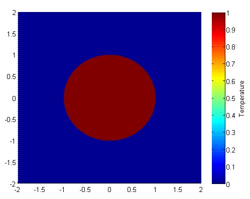
Let’s set up a specific example. A $4x4$ flat plate has a thermal diffusivity of $\alpha=.01$. The temperature is fixed at $u=1$ in an inner circle with radius $1$. Elsewhere, the initial temperature is $u=0$ and the outer boundaries are fixed at $u=0$ for all time. Find the temperature distribution over time.
(Note: I left off any units and have some simplified numbers for temperature and plate dimensions. Feel free to change them as you please, but make sure your formulation is still stable.)
The initial condition would look something like this:
Richardson Extrapolation Before we get started, it may help to glance at some of the basics of Richardson Extrapolation at Wikipedia.
The biggest challenge in our problem is that it requires a second derivative, which proves to be a little harder to compute with second order spatial accuracy. First and foremost, we can’t do it with just the two neighboring points (like we would be able to with evenly spaced points); we will need to use one more. Consider the points below. Assume that at each point $1,2,3,4$ we know the value of a function $f$ are $f_1,f_2,f_3,f_4$.
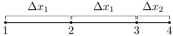
We will use information at the points $1,2,3,$ and $4$ to approximate the second derivative at point $3$, $f_3^{\prime\prime}$ . Why point $3$? In our particular problem, the second derivatives at points $1$ and $2$ can be approximated with a standard central difference and point $4$ will be a boundary, so the second derivative will not need to be calculated there.
Our first step will be to calculate the first derivatives at points $2,3,$ and $4$. These are fairly straightforward; we will use a central difference at point $2$ and Richardson extrapolation and points 3 and 4. They should look something like this \begin{eqnarray} f_2^{\prime} &=& \displaystyle\frac{f_3-f_1}{2\cdot \Delta x_1} \\ f_3^{\prime} &=& \displaystyle\frac{k_1\cdot (f_4-f_3)}{(k_1+1)\cdot \Delta x_2}+\frac{(f_3-f_2)}{(k_1+1)\cdot\Delta x_1} \\ f_4^{\prime} &=& \displaystyle\frac{k_2\cdot (f_4-f_3)}{(k_2-1)\cdot\Delta x_2}-\frac{f_4-f_2}{(k_2-1)\cdot (\Delta x_1+\Delta x_2) } \end{eqnarray} Where $k_1= \frac{ \Delta x_1}{ \Delta x_2}$ and $k_2=\frac{ \Delta x_1+ \Delta x_2}{ \Delta x_2}$ . Now we will use these to approximate the second derivative at $x_3$ with Richardson extrapolation. This is very similar to the formula except we will use a different value of $k$, namely $k_3=\frac{4\cdot k_1-1}{2\cdot k_1-2}$.
After wading through the algebra, your expression will simplify to $$f_3^{\prime\prime} = \frac{\Delta x_2^3\cdot (f_1-2 f_2+f_3)+\Delta x_1^3\cdot (6 f_4-6 f_3)+\Delta x_1^2\cdot \Delta x_2\cdot (-f_1+8 f_2-7 f_3)}{\Delta x_1^2\cdot \Delta x_2\cdot (\Delta x_1+\Delta x_2)\cdot (2 \Delta x_1+\Delta x_2)} $$
This is a pretty costly formula compared to the central difference method. Fortunately, we will not have to use this equation very often; only when the points are neighboring the boundary. Meanwhile, this allows us to use the cheap and effective central difference method at all other points. Therefore the overall computation should be fairly inexpensive.
We will also need to generate a mesh. Below is an example of the mesh. The elements have been triangulated for simple viewing in MATLAB, but there is no triangulation and no element formulation in the solution.
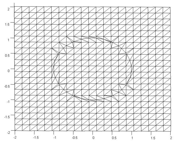
The original mesh here was a $22x22$ grid, but there were an additional 40 points added on the boundary to maintain the curvature of the circle. The important part is finding the $\Delta x_2$ and $\Delta y_2$ values for each of the points immediately neighboring a boundary and creating an additional point on the mesh.
When we loop through the mesh points we will ignore all points where the temperature is specified, use Richardson Extrapolation on the points adjacent to the 40 added points, and uses central differences elsewhere.
A Quick Look at Stability In the previous part we discussed stability, namely that in order for the old formulation to hold we needed to satisfy $$ \Delta t < \frac{\Delta x_1^2}{4\alpha}.$$ We will not perform a proper stability analysis, but our empirical results show that $$ \Delta t < \frac{\Delta x_1\cdot min(\Delta x_2)}{4\alpha}$$ is generally sufficient. Once you have your code written it is easy to empirically test different values of $\Delta t$.
The code
We are going to break it up into five steps: Create the Richardson extrapolation function, initialize relevant physical values, generate the mesh, set the boundary conditions, and set up the time loop. The time loop will consist of calculating the derivatives at each point, updating the temperature for each point, and then updating the visualization.
Step 1 Richardson Extrapolation
function [ddf3a] = richardson(dx1,dx2,f1,f2,f3,f4)
ddf3a = (dx2^3*(f1-2*f2+f3) + ...
         dx1^3*(6*f4-6*f3) + ...
         dx1^2*dx2*(-f1+8*f2-7*f3))...
       /(dx1^2*dx2*(dx1+dx2)*(2*dx1+dx2));
end
Step 2 Initialize variables
%Initialize Physical Values
dt=.01;                     %time step
nts=500;                    %number of time steps
alpha=.01;                  %thermal diffusivity
bounds=[-2 2 -2 2];         %corners of outer domain

%Mesh Variables
nx=50; ny=50;               %number of points in the x and y directions
%distance in between points
dx1=(bounds(2)-bounds(1))/(nx-1);
dy1=(bounds(4)-bounds(3))/(ny-1);
Step 3 Generate the Mesh
[xyz,skip,dx2,dy2,tri]=genmesh(bounds,nx,ny);

%The derivatives and temperature will be stored in a 1D arrays
nodes=length(skip);
uxx=zeros(nodes,1); uyy=zeros(nodes,1); T=zeros(nodes,1);
The function will return
- xyz: the nodes in a (np,2) where np is the number of points in the mesh.
- skip: an array that shows whether a point is on a boundary or neighboring one.
- dx2 and dy2: maps relating the distance from a point to the boundary if it neighbors the boundary.
- tri the “connectivity" of the mesh.
An alternative to creating your own tri connectivity would be using the MATLAB built in function tri=delaunay(x,y) but it will not look as good as if you make it yourself.
I will not include any of the code in this post (my version is 160 lines long and it is mostly boring) but you can access the text here.
Step 4 Apply Initial and Boundary Conditions
for p=1:length(skip)
    if skip(p) < 0
        u(p)=1.0;
    else
        u(p)=0.0;
    end
end
Step 5 Time Loop The time loops has three components, first calculate the second derivatives, then update temperature, then update the visualization.
One note before we get into the code. We are using the MATLAB function “bitget” which determines based of the values of skip(p) (see Step 3) whether it is close to the boundary. This is by all means not necessarily the best way to determine whether a point neighbors a boundary, but it works and is not too costly.
for t=1:nts
    for i=2:ny-1
        for j=2:nx-1
            p=nx*(i-1)+j;
            if skip(p) < 0
                continue
            end
            if     bitget(skip(p),1)==1
                uxx(p)=richardson(dx1,abs(dx2(p)),u(p-2),u(p-1),u(p),T_b);
            elseif bitget(skip(p),3)==1
                uxx(p)=richardson(dx1,abs(dx2(p)),u(p+2),u(p+1),u(p),T_b);
            else
                uxx(p)=(u(p-1)-2*u(p)+u(p+1))/dx1^2;
            end

            if     bitget(skip(p),2)==1
                uyy(p)=richardson(dy1,abs(dy2(p)),u(p-2*nx),u(p-nx),u(p),T_b);
            elseif bitget(skip(p),4)==1
                uyy(p)=richardson(dy1,abs(dy2(p)),u(p+2*nx),u(p+nx),u(p),T_b);
            else
                uyy(p)=(u(p-nx)-2*u(p)+u(p+nx))/dy1^2;
            end
        end
    end

    for i=2:nx-1
        for j=2:ny-1
            p=nx*(i-1)+j;
            if skip(p)<0
                continue
            end
            u(p)=u(p)+alpha*dt*(uxx(p)+uyy(p));
        end
    end
    trisurf(tri,xyz(:,1),xyz(:,2),u,'FaceColor','interp');
    frame = getframe(1);
end
Results
Below are two animations of the temperature distribution over time.
Some notes about the code
If you are a novice programmer, you may not have heard of maps. Maps are "objects with keys that index to values" (see here and here). They are similar to an array, except that keys must be unique, keys don't need to be integers, and key values typically aren't ordered. A map is by no means necessary here, but it is an efficient way to store and quickly retrieve the $\Delta x_2$ and $\Delta y_2$ values.
The most confusing part of the code above is implementation of the skip array with bitget. Basically, skip is an array with an integer for every node.
- If a node p is on or inside the circle, skip(p)=-1.
- If it is outside the circle and not adjacent to it, skip(p)=0.
- If it is adjacent to the circle (left, below, right, above) then we add 1,2,4,8 respectively to skip(p). For example, if a point is below and to the right of points on the circle, then skip(p)=6.
We can then reverse engineer skip(p) with bitget. This is not necessarily the best or only way, but it is a relatively simple implementation.
You can save some space in memory by letting uxx and uyy be single values instead of arrays. This however, would either require two arrays for temperature (an old and a new) or some algorithm to keep from overwriting old values of temperature before all derivatives are calculated. Since we are dealing with a relatively coarse 2D mesh, this is not a significant issue.